Online Reinforcement Learning
In this post, I try to summarize some interesting online RL algorithms.
Online Reinforcement Learning
In this post I will overview different single and multi-agent online Reinforcement Learning (RL) algorithms. By online I mean the algorithms that can interact with an environment and collect data, in contrast to offline RL. I will update this post and add algorithms periodically.
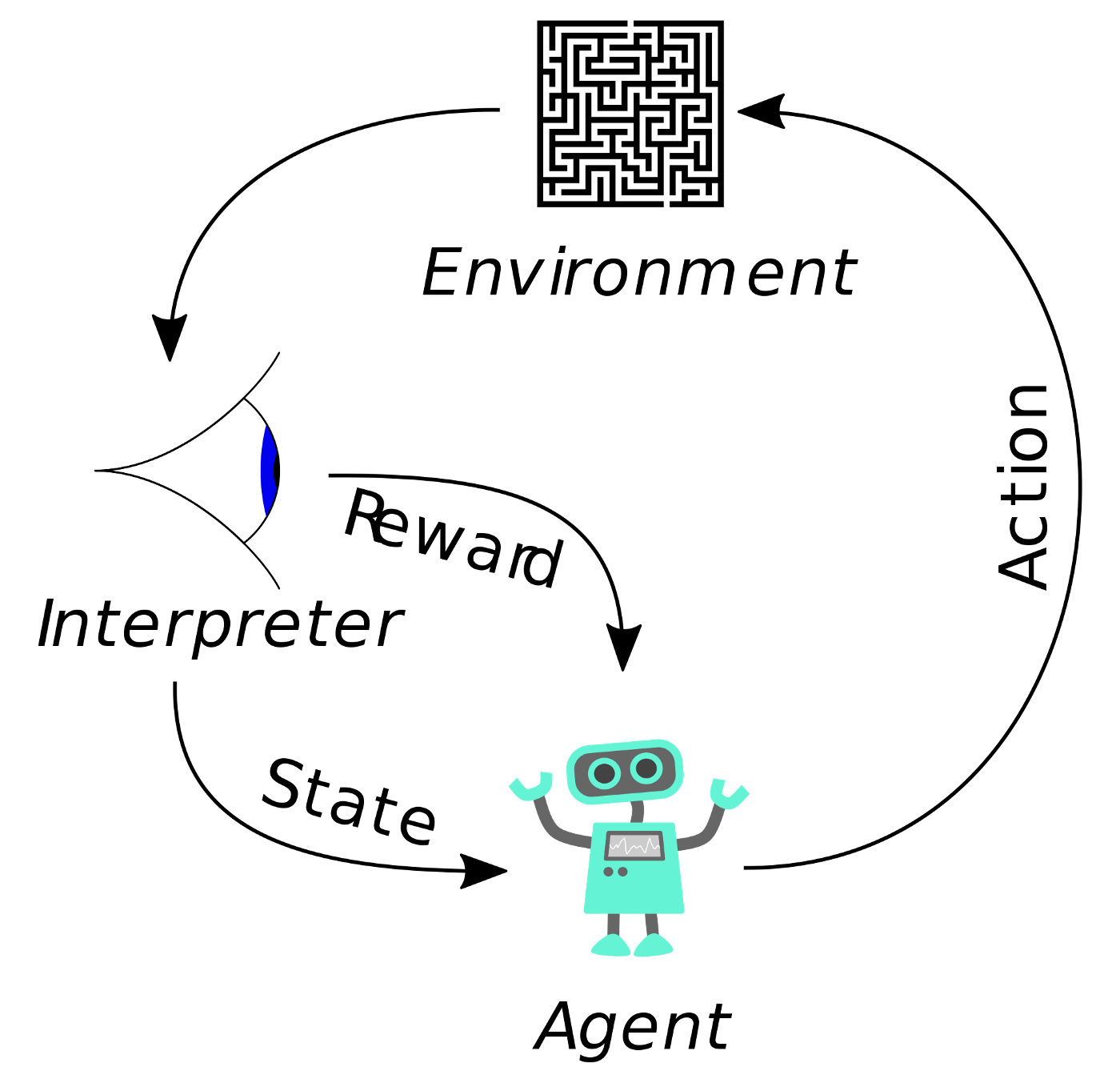 RL diagram
Here are some resources to learn more about RL!
-
David Silver’s course
-
CS287 at UC Berkeley - Advanced Robotics course - Instructor: Pieter Abbeel
-
CS 285 at UC Berkeley - Deep Reinforcement Learning course - Instructor: Sergey Levine
-
CS234 at Stanford - Reinforcement Learning course - Instructor: Emma Brunskill
-
CS885 at University of Waterloo - Reinforcement Learning course - Instructor: Pascal Poupart
-
Arthur Juliani’s posts
-
Jonathan Hui’s posts
-
A Free course in Deep Reinforcement Learning from beginner to expert by Thomas Simonni
Single agent
DQN
We will take a look at DQN with experience replay buffer and the target network.
DQN is a value-based method. It means that we try to learn a value function and then use it to achieve the policy. In DQN we use a neural network as a function approximator for our value function. It gets the state as input and outputs the value for different actions in that state. These values are not limited to be between zero and one, like probabilities, and can have other values based on the environment and the reward function we define.
DQN is an off-policy method which means that we are using data from old policies, the data that we gather in every interaction with the environment and save it in the experience replay buffer, to sample from it later and train the network. The size of the replay buffer should be large enough to reduce the $i.i.d$ property between data that we sample from it.
To use DQN, the action should be discrete. We can use it for continuous action spaces by discretizing the action space, but it’s better to use other techniques that can handle continuous action spaces such as Policy Gradients. First, let’s see the algorithm’s sudo code:

In this algorithm, we have experience replay buffer and a target network with a different set of parameters that will be updated every $C$ steps. These tricks help to get a better and more stable method rather than pure DQN. There are a lot of improvements for DQN and we will see some of them in the next posts too.
First, we initialize the weights of both networks and then start from the initial state s and take action a with epsilon-greedy policy. In the epsilon-greedy policy, we select an action a randomly or using the Q-network. Then we execute the selected action and get the next state, reward, and the done values from the environment and save them in our replay buffer. Then we sample a random batch from the replay buffer and calculate target based on the Bellman equation in the above picture and use MSE loss and gradient descent to update the network weights. We will update the weights of our target network every $C$ steps.
In the training procedure, we use epsilon decay. It means that we consider a big value for epsilon, such as $1$. Then during the training procedure, as we go forward, we reduce its value to something like $0.02$ or $0.05$, based on the environment. It will help the agent to do more exploration in the first steps and learn more about the environment. It’s better to have some exploration always. That’s a trade-off between exploration-exploitation. In test time, we have to use a greedy policy. It means we have to select the action with the highest value, not randomly anymore (set epsilon to zero actually).
REINFORCE
REINFORCE is a Monte-Carlo Policy Gradient (PG) method. In PGs, we try to find a policy to map the state into action directly.
In value-based methods, we find a value function and use it to find the optimal policy. Policy gradient methods can be used for stochastic policies and continuous action spaces. If you want to use DQN for continuous action spaces, you have to discretize your action space. This will reduce the performance and if the number of actions is high, it will be difficult and impossible. But REINFORCE algorithms can be used for discrete or continuous action spaces. They are on-policy because they use the samples gathered from the current policy.
There are different versions of REINFORCE. The first one is without a baseline. It is as follows:

In this version, we consider a policy (here a neural network) and initialize it with some random weights. Then we play for one episode and after that, we calculate discounted reward from each time step towards the end of the episode. This discounted reward (G in the above sudo code) will be multiplied by the gradient. This G is different based on the environment and the reward function we define. For example, consider that we have three actions. The first action is a bad action and the other two actions are some good actions that will cause more future discounted rewards. If we have three positive G values for three different actions, we are pushing the network towards all of them. Actually, we push the network towards action number one slightly and towards others more. Now consider we have one negative G value for the first action and two G values for the other two actions. Here we are pushing the network far from the first action and towards the other two actions. You see?! the value of G and its sign is important. It guides our gradient direction and its step size. To solve such problems, one way is to use baseline. This will reduce the variance and accelerate the learning procedure. For example, subtract the value of the state from it, or normalize it with the mean and variance of the discounted reward of the current episode. You can see the sudo code for REINFORCE with baseline in the following picture:

In this version, first, we initialize the policy and value networks. It is possible to use two separate networks or a multi-head network with a shared part. Then we play an episode and calculate the discounted reward from every step until the end of the episode (reward to go). Then subtract the value (from the learned neural net) for that state from the discounted reward (REINFORCE with baseline) and use it to update the weights of value and policy networks. Then generate another episode and repeat the loop.
In the Sutton&Barto book, they do not consider the above algorithm as actor-critic (another RL algorithm that we will see in the next posts). It learns the value function but it is not used as a critic! I think it is because we do not use the learned value function (critic) in the first term of the policy gradient rescaler (for bootstrapping) to tell us how good is our policy or action in every step or in a batch of actions (in A2C and A3C we do the update every t_max step). In REINFORCE we update the network at the end of each episode.
“The REINFORCE method follows directly from the policy gradient theorem. Adding a state-value function as a baseline reduces REINFORCE’s variance without introducing bias. Using the state-value function for bootstrapping introduces bias but is often desirable for the same reason that bootstrapping TD methods are often superior to Monte Carlo methods (substantially reduced variance). The state-value function assigns credit to — critizes — the policy’s action selections, and accordingly the former is termed the critic and the latter the actor, and these overall methods are termed actor–critic methods. Actor–critic methods are sometimes referred to as advantage actor–critic (“A2C”) methods in the literature.” [Sutton&Barto — second edition]
I think Monte-Carlo policy gradient and Actor-Critic policy gradient are good names as I saw in the slides of David Silver course.

I also saw the following slide from the Deep Reinforcement Learning and Control course (CMU 10703) at Carnegie Mellon University:

Here they consider every method that uses value function (V or Q) as actor-critic and if you just consider reward to go in the policy gradient rescaler, it is REINFORCE. The policy evaluation by the value function can be TD or MC.
Summary of the categorization:
-
Vanilla REINFORCE or Policy gradient → we use G as gradient rescaler.
-
REINFORCE with baseline → we use $\frac{G-mean(G)}{std(G)}$ or $(G-V)$ as gradient rescaler. We do not use $V$ in $G$. $G$ is only the reward to go for every step in the episode → $G_t = r_t + \gamma r_{t+1} + … $
-
Actor-Critic → we use $V$ in the first term of gradient rescaler and call it Advantage ($A$):
$A_t = Q(s_t, a_t) - V(s_t)$
$A_t = r_t + \gamma V_{s_{t+1}} - V_{s_t}$ → for one-step
$A_t = r_t + \gamma r_{t+1} + \gamma^2 V_{s_{t+2}} - V_{s_t}$ → for 2-step
and so on.
- In Actor-Critics you can do the update each $N$ step based on your task. This $N$ can be less than an episode.
Anyway, let’s continue.
This algorithm can be used for either discrete or continuous action spaces. In discrete action spaces, it will output a probability distribution over action, which means that the activation function of the output layer is a softmax. For exploration-exploitation, it samples from the actions based on their probabilities. Actions with higher probabilities have more chances to be selected.
In continuous action spaces, the output will not have any softmax. Because the output is a mean for a normal distribution. We consider one neuron for each action and it can have any value. In fact, the policy is a normal distribution and we calculate its mean by a neural network. The variance can be fixed or decrease over time or can be learned. You can consider it as a function of the input state, or define it as a parameter that can be learned by gradient descent. If you want to learn the sigma too, you have to consider the number of actions. For example, if we want to map the front view image of a self-driving car into steering and throttle-brake, we have two continuous actions. So we have to have two mean and two variance for these two actions. During training, we sample from this normal distribution for exploration of the environment, but in the test, we only use the mean as action.
A2C
A3C
PPO
DDPG
This algorithm is from the “Continuous Control with Deep Reinforcement Learning” paper and uses the ideas from deep q-learning in the continuous action domain and is a model-free method based on the deterministic policy gradient.
In Deterministic Policy Gradient (DPG), for each state, we have one clearly defined action to take (the output of policy is one value for action and for exploration we add a noise, normal noise for example, to the action). But in Stochastic Gradient Descent, we have a distribution over actions (the output of policy is mean and variance of a normal distribution) and sample from that distribution to get the action, for exploration. In another term, in stochastic policy gradient, we have a distribution with mean and variance and we draw a sample from that as an action. When we reduce the variance to zero, the policy will be deterministic.
When the action space is discrete, such as q-learning, we get the max over q-values of all actions and select the best action. But in continuous action spaces, you cannot apply q-learning directly, because in continuous spaces finding the greedy policy requires optimization of $a_t$ at every time-step and would be too slow for large networks and continuous action spaces. Based on the proposed equation in the reference paper, here we approximate max Q(s, a) over actions with Q(a, µ(s)).
In DDPG, they used function approximators, neural nets, for both action-value function $Q$ and deterministic policy function $\mu$. In addition, DDPG uses some techniques for stabilizing training, such as updating the target networks using soft updating for both $\mu$ and $Q$. It also uses batch normalization layers, noise for exploration, and a replay buffer to break temporal correlations.
This algorithm is an actor-critic method and the network structure is as follows:

First, the policy network gets the state and outputs the action mean vector. This will be a vector of mean values for different actions. For example, in a self-driving car, there are two continuous actions: steering and acceleration&braking (one continuous value between $-x$ to $x$, the negative values are for braking and positive values are for acceleration). So we will have two mean for these two actions. To consider exploration, we can use Ornstein-Uhlenbeck or normal noise and add it to the action mean vector in the training phase. In the test phase, we can use the mean vector directly without any added noise. Then this action vector will be concatenated with observation and fed into the $Q$ network. The output of the $Q$ network will be one single value as a state-action value. In DQN, because it had discrete action space, we had multiple state-action values for each action, but here because the action space is continuous, we feed the actions into the $Q$ network and get one single value as the state-action value.
Finally, the sudo code for DDPG is as follows:

To understand the algorithm better, it’s good to try to implement it and play with its parameters and test it in different environments. Here is a good implementation in PyTorch that you can start with this.
I also found the Spinningup implementation of DDPG very clear and understandable too. You can find it here
For POMDP problems, it is possible to use LSTMs or any other RNN layers to get a sequence of observations. It needs a different type of replay buffer for sequential data.
SAC
Ape-X
R2D2
IMPALA
Never Give-Up
Agent57
Multi-Agent
In Multi-Agent Reinforcement Learning (MARL)problems, there are several agents who usually have their own private observation and want to take an action based on that observation. This observation is local and different from the full state of the environment in that time-step. The other problem that we face in such environments is the non-stationary problem because all agents are learning and their behavior would be different during training as they learn to act differently.
To solve this problem, the most naive approach is to use single-agent RL algorithms for each agent and treat other agents as part of the environment. Some methods like Independent Q-Learning (IQL) work fine in some multi-agent RL problems in practice but there is no guarantee for them to converge. In IQL, each agent has one separate action-value function that gets the agent’s local observation to select its action based on that. It is also possible to use additional inputs like previous actions as input. Usually, in partially observable environments, we use RNNs to consider a history of several sequential observation-actions.

The other approach is to have a fully centralised method to learn and act in a centralised fashion. We can consider this type as a big single-agent problem. This approach is also valid in some problems that you don’t need decentralised execution. For example for traffic management or traffic light management, it is possible to use such approaches.
There is one more case that is somewhere between the previous two ones: centralised training and decentralised execution. Usually in the training procedure, because we train agents in a simulation environment or in a lab, we have access to the full state and information in the training phase. So it is better to use this knowledge. On the other hand, the learned policy should be decentralised in some environments and agents cannot have access to the full state during the execution phase. So having algorithms to use the available knowledge in the training phase and learn a policy that is not dependent on the full state in the execution time is necessary. Here we focus on the last case.
There are several works that try to propose such an algorithm and can be divided into two groups:
-
value-based methods like Value Decomposition Networks (VDN) and QMIX
-
actor-critic methods like MADDPG and COMA
VALUE-BASED METHODS
These approaches try to propose a way to be able to use value-based methods like Q-learning and train them in a centralised way and use them for decentralised execution.
VDN
This work proposes a way to have separate action-value functions for multiple agents and learn them by just one shared team reward signal. The joint action-value function is a linear summation of all action-value functions of all agents. Actually, by using a single shared reward signal, it tries to learn decomposed value functions for each agent and use it for decentralised execution.

Consider a case with 2 agents, the reward would be:

Then the total $Q$ function is:
It is using the same Bellman equation to standard q-learning approach and just replaces $Q$ in that equation with the new $Q$ value.
QMIX
QMIX is somehow an extension to value decomposition networks (VDN) but tries to mix the Q-value of different agents in a nonlinear way. They use global state $s_t$ as input to hypernetworks to generate weights and biases of the mixing network.

Here again, the equation to update the weights is the standard Bellman equation in which the $Q$ is replaced with $Q_tot$ in the above figure.
ACTOR-CRITIC BASED METHODS
This group of methods tries to use actor-critic architecture to do centralised training and decentralised execution. Usually, they use the full state and additional information which are available in the training phase in the critic network to generate a richer signal for the actor.
MADDPG
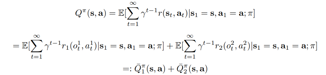
Multi-Agent DDPG (MADDPG) is a method to use separate actors and critics for each agent and train the critic in a centralised way and use the actor in execution. So each agent has one actor and one critic. The actor has access to its own action-observation data and is trained by them and the critic has access to observation and action of all agents and is trained by all of them.

The centralised action-value function for each agent can be written as:

And the gradient can be written as follows:

As you see, the policy is conditioned on the observation of the agent itself, o_i, and the critic is conditioned on the full state and actions of all agents. This separate critic for each agent allows us to have agents with different rewards, cooperative or competitive behaviors.
COMA
The talk can be found here.
Counterfactual Multi-Agent (COMA) policy gradient is a method for cooperative multi-agent systems and uses a centralised critic to estimate the Q-function and decentralised actors to optimise the agents’ policies. In addition, to address the problem of multi-agent credit assignment, it uses a counterfactual baseline that marginalises out a single agent’s action, while keeping the other agents’ actions fixed. The idea comes from difference rewards, in which each agent learns from a shaped reward $D_a = r(s, u) − r(s,(u^{-a}, c_a))$ that compares the global reward to the reward received when the action of agent $a$ is replaced with a default action $c_a$.
COMA also uses a critic representation that allows the counterfactual baseline to be computed efficiently in a single forward pass.

For each agent $a$, we can then compute an advantage function that compares the Q-value for the current action $u^a$ to a counterfactual baseline that marginalizes out $u^a$, while keeping the other agents’ actions $u^{-a}$ fixed:
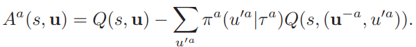
In contrast to MADDPG, COMA is an on-policy approach and has only one critic network.