This post is a summary (almost!) of the model-based RL tutorial at ICML-2020 by Igor Mordatch and Jess Hamrick. You can find the videos here. The pictures are from the slides in the talk.

Introduction and Motivation

Having access to a world model, and using it for decision-making is a powerful idea. There are a lot of applications of MBRL in different areas like robotics (manipulation- what will happen by doing an action), self-driving cars (having a model of other agents decisions and future motions and act accordingly), games (AlphaGo- search over different possibilities), Science ( chemical use-cases), and operation research and energy applications (allocate renewable energy at different points in time to meet the demand).

Problem Statement

In sequential decision making, the agent will interact with the world by doing action $a$ and getting the next state $s$ and reward $r$.

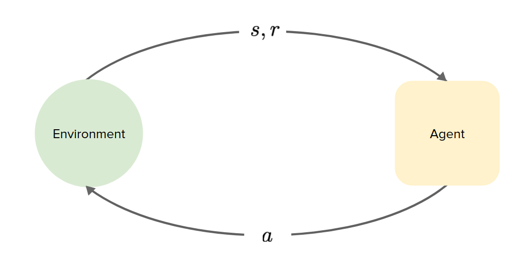
We can write this problem as a Markov Decision Process (MDP) as follows:

States $S \epsilon R^{d_S}$
Actions $A \epsilon R^{d_A}$
Reward function $R: S \times A \rightarrow R$
Transition function $T: S \times A \rightarrow S$
Discount $\gamma \epsilon (0,1)$
Policy $\pi: S \rightarrow A$

The goal is to find a policy which maximizes the sum of discounted future rewards: $$ \text{argmax}_{\pi} \sum_{t=0}^\infty \gamma^t R(s_t, a_t) $$ subject to $$ a_t = \pi(s_t) , s_{t+1}=T(s_t, a_t) $$

How to solve this optimization problem?!

Collect data $D= \{ s_t, a_t, r_{t+1}, s_{t+1} \}_{t=0}^T$.
Model-free: learn policy directly from data

$$ D \rightarrow \pi \quad \text{e.g. Q-learning, policy gradient}$$

Model-based: learn model, then use it to learn or improve a policy

$$ D \rightarrow f \rightarrow \pi$$

What is a model?

a model is a representation that explicitly encodes knowledge about the structure of the environment and task.

This model can take a lot of different forms:

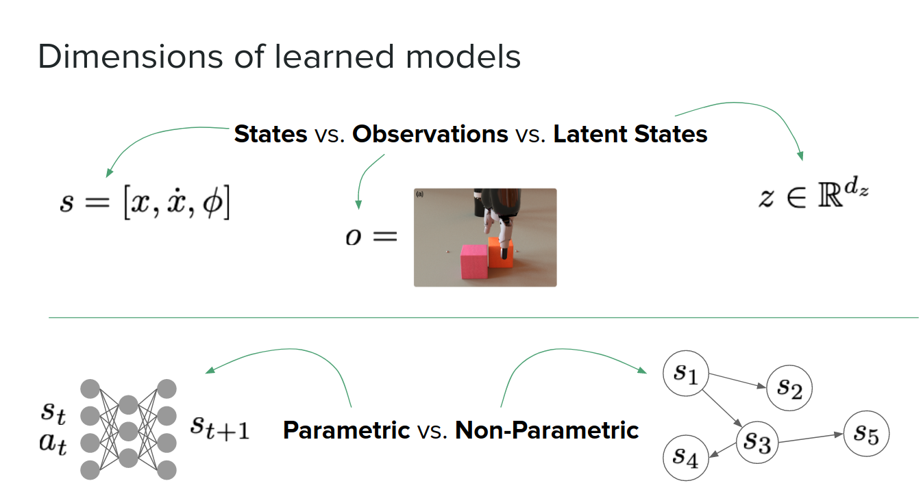
A transition/dynamic model: $s_{t+1} = f_s(s_t, a_t)$
A model of rewards: $r_{t+1} = f_r(s_t, a_t)$
An inverse transition/dynamics model (which tells you what is the action to take and go from one state to the next state): $a_t = f_s^{-1}(s_t, s_{t+1})$
A model of distance of two states: $d_{ij} = f_d(s_i, s_j)$
A model of future returns: $G_t = Q(s_t, a_t)$ or $G_t = V(s_t)$

Typically when someone says MBRL, he/she means the firs two items.

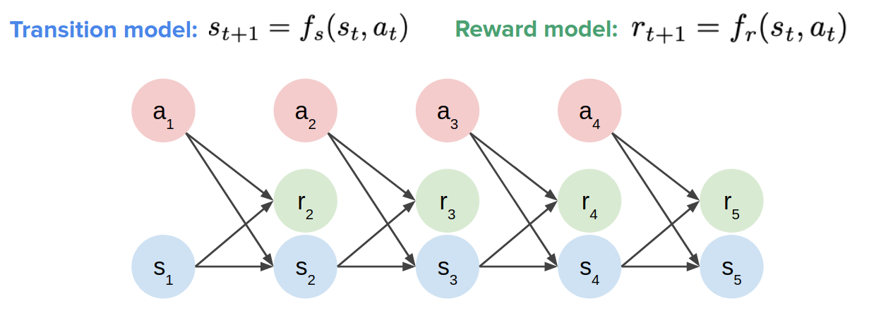
Sometimes we know the ground truth dynamics and rewards. Might as well use them! Like game environments or simulators like Mujoco, Carla, and so on.

But we don't have access to the model in all cases, so we need to learn the model. In cases like in robots, complex physical dynamics, and interaction with humans.

How to use a model?

In model-free RL agent, we have a policy and learning algorithm like the figure below:

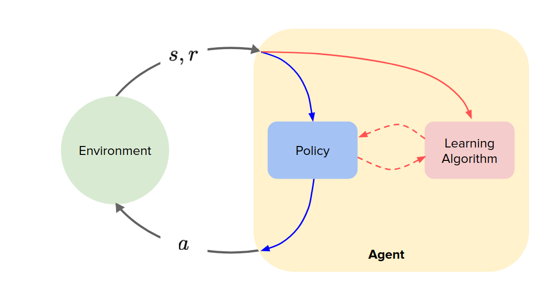
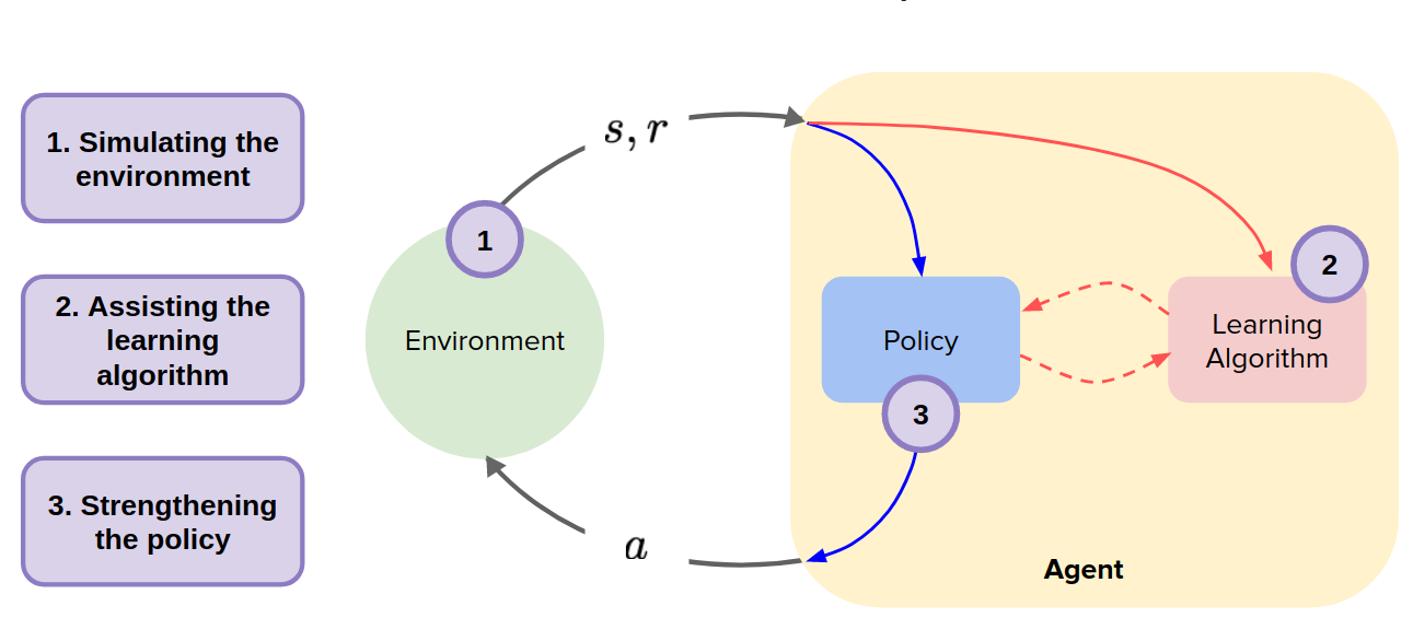
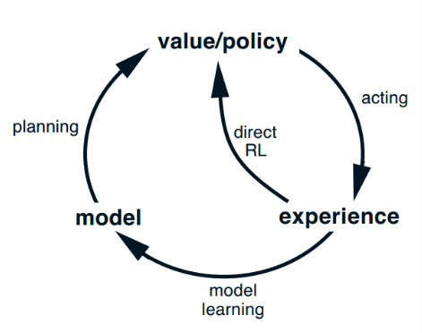
In model-based RL we can use the model in three different ways:

simulating the environment: replacing the environment with a model and use it to generate data and use it to update the policy.
Assisting the learning algorithm: modify the learning algorithm to use the model to interpret the data it is getting differently.
Strengthening the policy: allow the agent at test time to use the model to try out different actions before it commits to one of them (taking action in the real world).

In general, to compare model-free and model-based:

How to learn a model?

Two different dimensions are useful to pay attention to:

representation of the features for the states that the model is being learned over them
representation of the transition between states

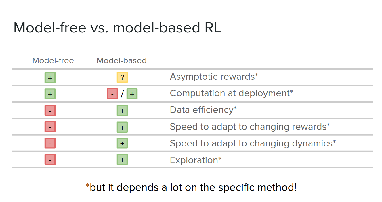
To continue, we take a look at different transition models.

state-transition models

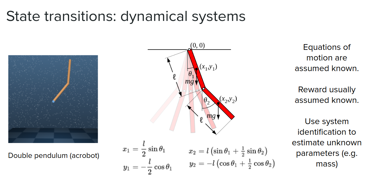
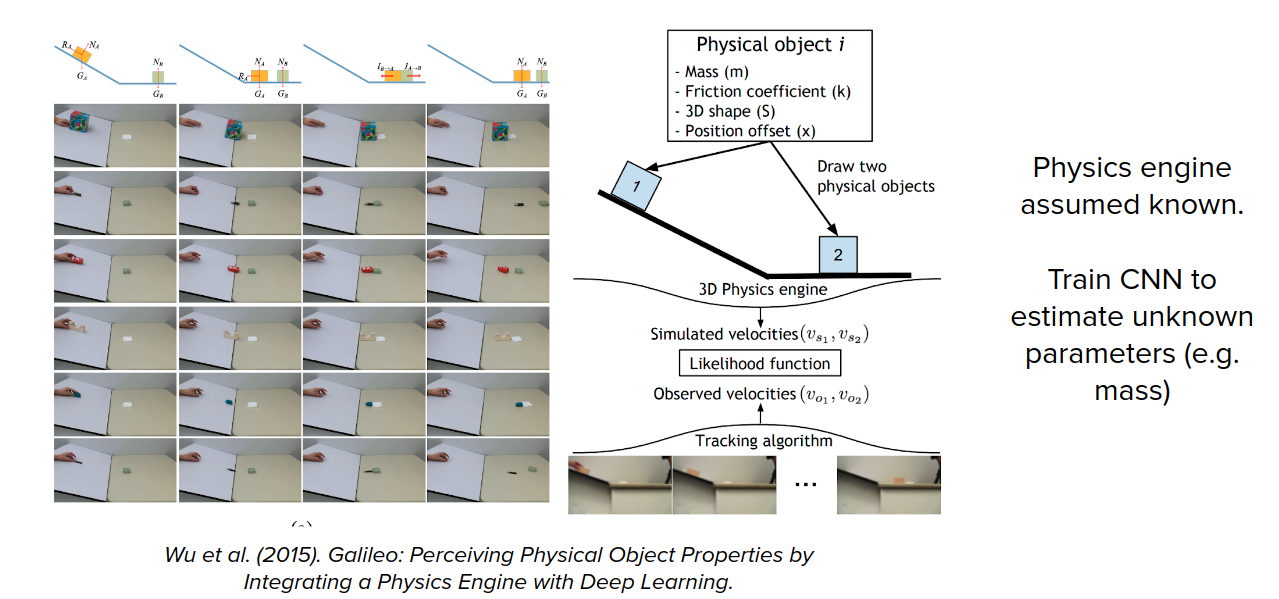
We know equations of motion and dynamics in some cases, but we don't know the exact parameters like mass. We can use system identification to estimate unknown parameters like mass. But these sorts of cases require having a lot of domain knowledge about how exactly the system works.

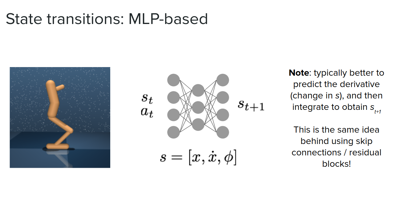
In some cases that we don't know the dynamics of motion, we can use an MLP to get a concatenation of $s_t, a_t$, and output the next state $s_{t+1}$.

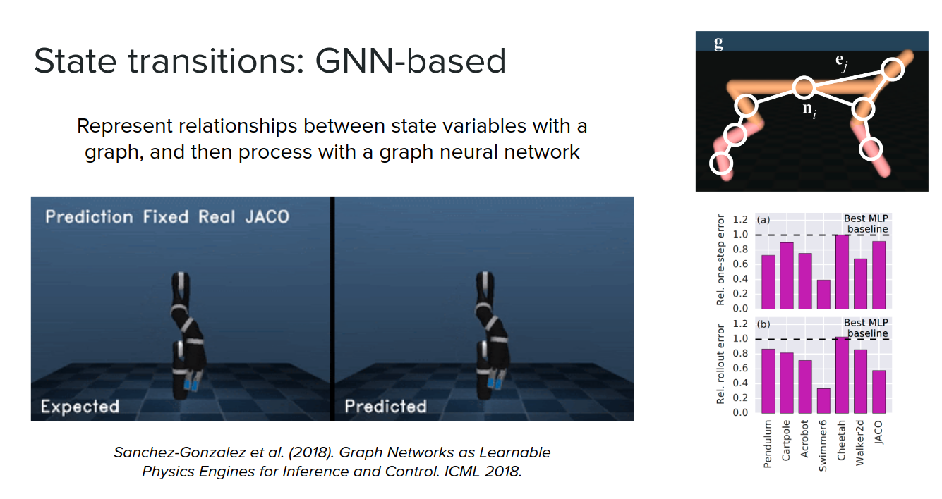
In cases that we have some, not perfect, domain knowledge about the environment, we can use graph neural networks (GNNs) to model the agent (robot). For example, in Mujoco, we can model a robot (agent) with nodes as its body parts and edges as joint and learn the physics engine.

observation-transition models

In these cases, we don't have access to states (low-level states like joint angles), but we have access to images. The MDP for these cases would be like this:

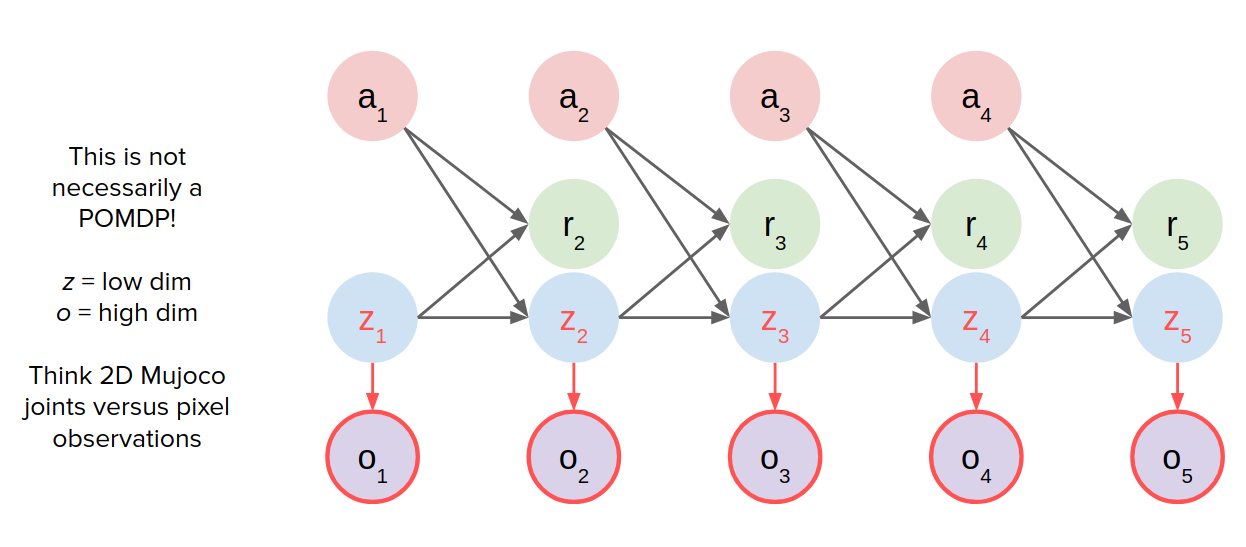
So what can we do with this?

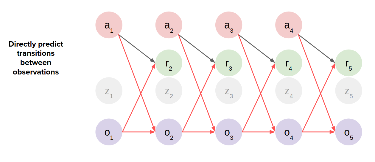
Directly predict transitions between observations (observation-transition models)

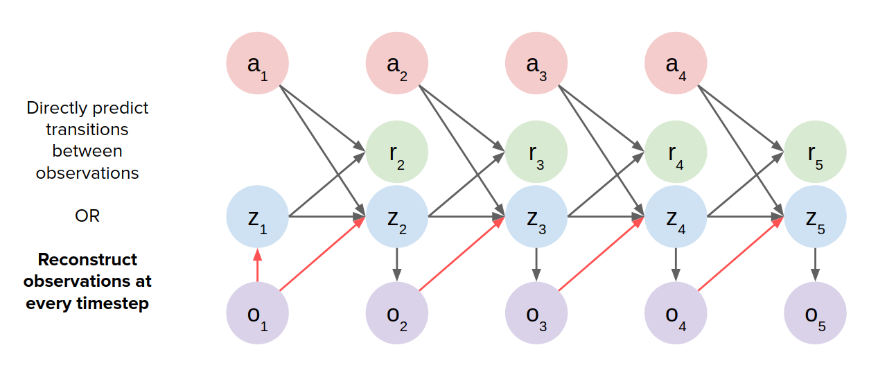
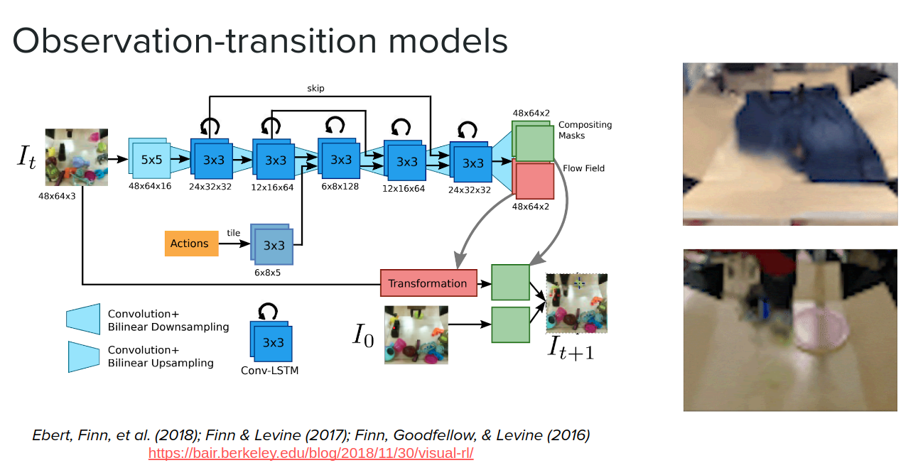
Reconstruct observation at every timestep: Using sth like LSTMs. Here we need to reconstruct the whole observation in each timestep. The images can be blurry in these cases.

latent state-transition models

Another option when we have just access to observation is to instead of making transition between observations we can infere a latent state and then make transitions in that latent space (latent state-transition models) not in the observation space. It would be much faster than reconstructing the observation on every timestep. We take our initial observation or perhaps the last couple of observations and embed them into the latent state and then unroll it in time and do predictions in $z$ instead of $o$.

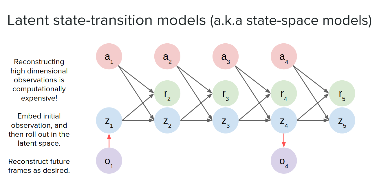
Usually we use the observation and reconstruct it during training but at test time we can unroll it very quickly. we can also reconstruct observation at each timestep we want (not necessarily in all timesteps).

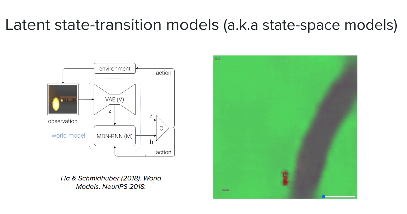
Structured latent state-transition models

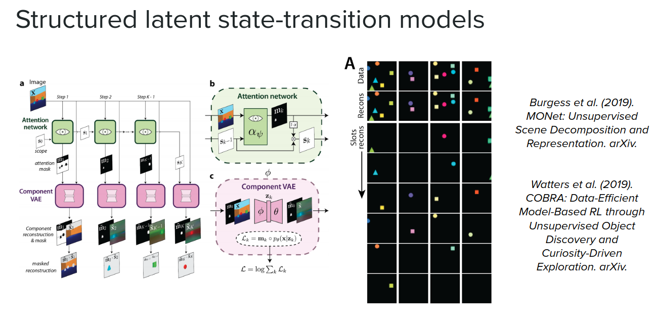
Another thing that you can do if you have a little bit more domain knowledge is to add a little bit of structure into your latent state. For example, if you know that the scene that you are trying to model consists of objects, you can try to actually explicitly detect those objects, segment them out and then learn those transitions between objects.

Recurrent value models

The idea is that when you unroll your latent-state, you additionally predict the value of the state at each point of the future, in addition to reward. We can train the model without necessarily needing to train using observations, but just training it by predicting the value progressing toward actual observed values when you roll it out in the real environment.

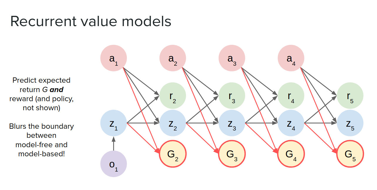
Why is this useful? Because some types of planners only need you to predict values rather than predicting states like MCTS (Monte Carlo tree search).

Non-Parametric models

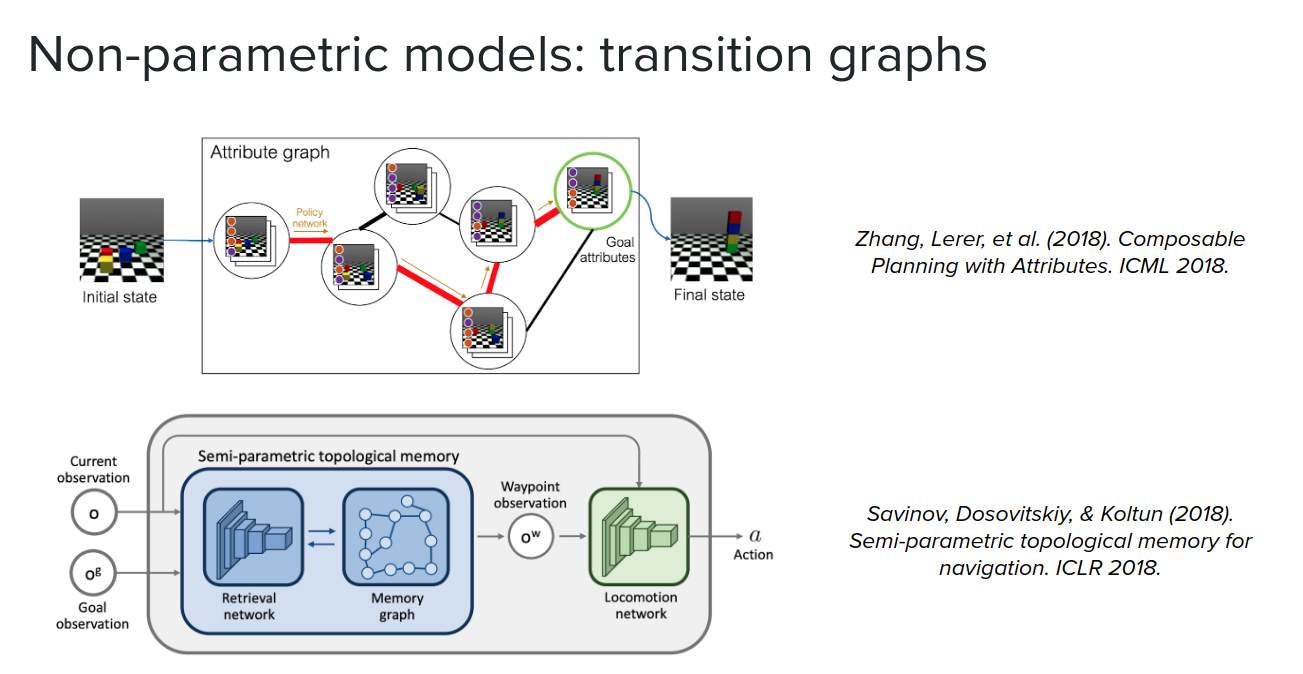
So far, we talked about parametric ways of learning the model. We can also use non-parametric methods like graphs.

For example, the replay buffer that we use in off-policy methods can be seen as an approximation to a type of model, where if you have enough data in your replay buffer, you can sample from the buffer and basically access the density model over your transitions. You can use extra replay to get the same level performances you would get using a model-based method that learns a parametric model.

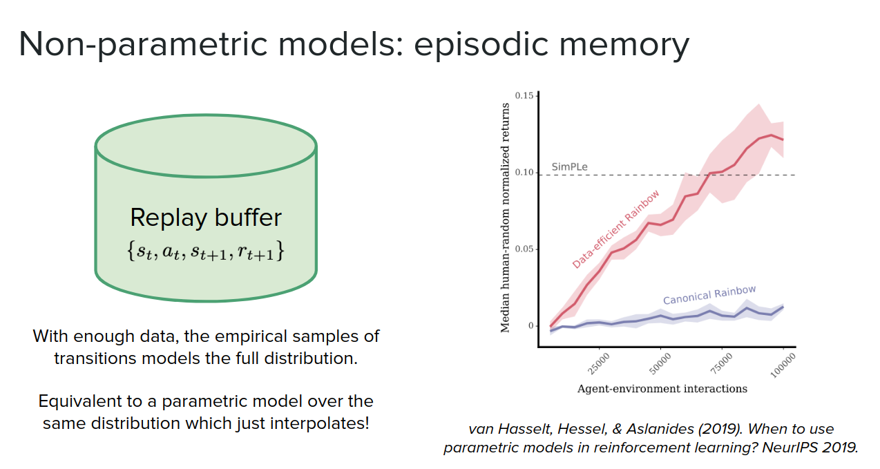
We can also use data in the buffer to use data points and learn the transition between them and interpolate to find states between those states in the buffer. Somehow learning distribution and use it to generate new data points.

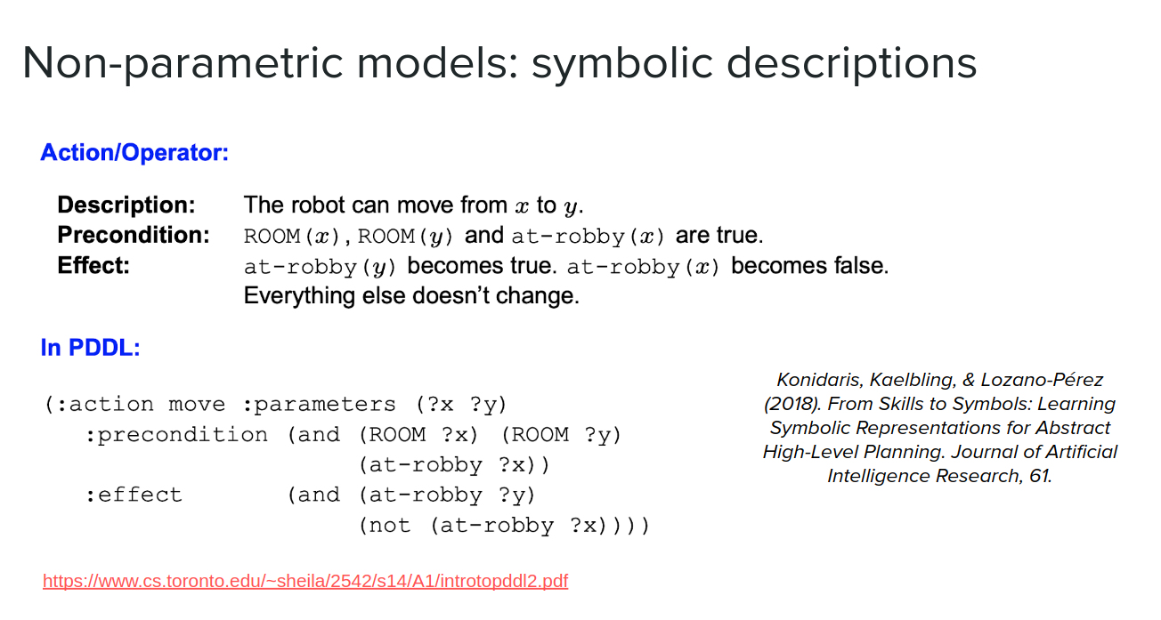
Another form of non-parametric transition is a symbolic description popular in the planning community, not in the deep learning community.

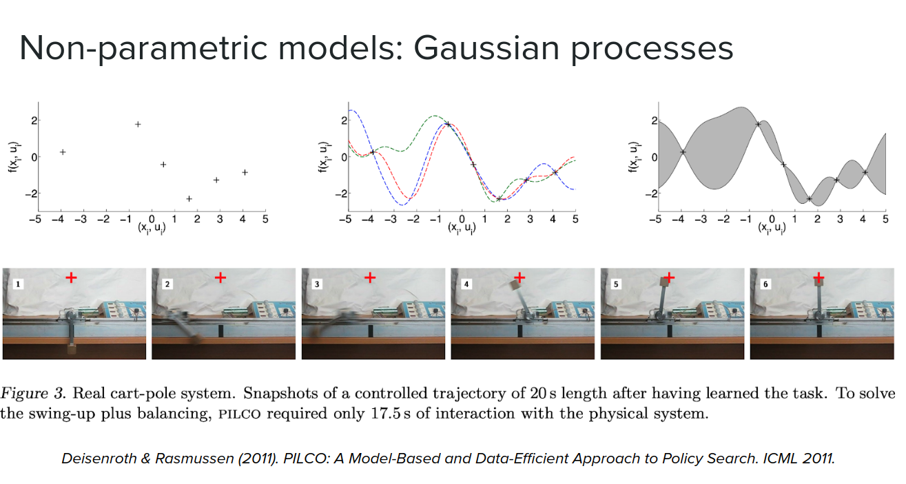
The other form of non-parametric models is gaussian processes, which give us strong predictions using a very small amount of data. PILCO is one example of these algorithms.

Model-based control and how to use a model?

We will be using this landscape of various methods and categories that exist, including some representative algorithms:

As we saw earlier, we can use the model in three different ways. In continue, we will see some examples of each case.

Simulating the environment

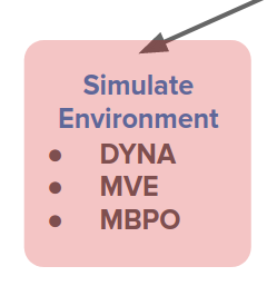
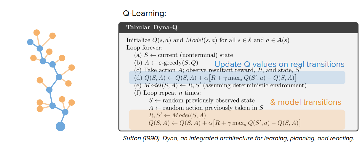
One way is to mix the real data with model-generated experience and then apply traditional model-free algorithms like Q-learning, policy gradient, etc. In these cases, the model offers a larger and augmented training dataset.

Dyna-Q is an example that uses Q-learning with a learned model. Dyna does the traditional Q-learning updates on real transitions and uses a model to create fictitious imaginary transitions from the real states and perform exactly the same Q-learning updates on those. So it's basically just a way to augment the experience.

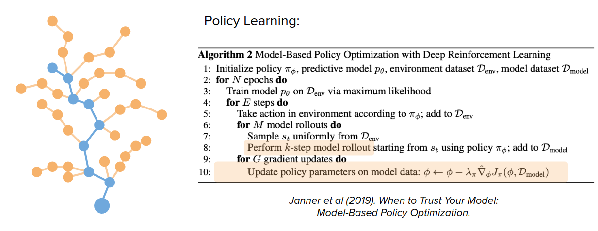
This can also be applied to policy learning. We don't need to perform just a single step but multiple steps according to the model to generate experience even further away from the real data and do policy parameter updates entirely on these fictitious experiences.

Assisting the learning algorithm

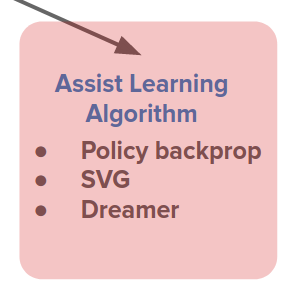
One important way that this can be done is to allow end-to-end training through our models. End-to-end training has recently been very successful in improving and simplifying supervised learning methods in computer vision, NLP, etc.

The question is, "can we apply the same type of end-to-end approaches to RL?"

One example is just the policy gradient algorithm. Let's say we want to maximize the sum of the discounted future reward of some parametric policy. We can write the objective function with respect to the policy parameters $\theta$

$$ J(\theta) = \sum_{t=0}^{\infty} \gamma^t R(s_t, a_t) , \quad a_t = \pi_{\theta}(s_t) , \quad s_{t+1} = T(s_t, a_t) $$

Now we need to apply gradient ascent (for maximization) on policy gradient with respect to policy parameters $\theta \rightarrow \nabla_{\theta}J$.

So how can we calculate this $\nabla_{\theta}J$ ?

Sampling-based methods have been proposed, like REINFORCE, to estimate this gradient. But the problem with them is that they can have very high variance and often require the policy to have some randomness to make decisions. This can be unfavorable.

The next solution is when we have accurate and smooth models. Accurate and smooth models, aside from imaginary experiences, offer derivatives:

$$ s_{t+1} = f_s(s_t, a_t) \quad r_t = f_r(s_t, a_t) $$$$ \nabla_{s_t}(s_{t+1}), \quad \nabla_{a_t}(s_{t+1}), \quad \nabla_{s_t}(r_t), \quad \nabla_{a_t}(r_t), \quad ... $$

And they are able to answer questions such as: how do small changes in action change next state or reward any of other quantities?

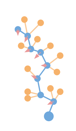
Why is this useful? This is useful because it will allow us to do this type of end-to-end differentiation algorithms like back-propagation.

Let's rewrite our objective function using models:

$$ J(\theta) \approx \sum_{t=0}^{H} \gamma^t r_t , \quad a_t = \pi_{\theta}(s_t) , \quad s_{t+1} = f_s(s_t, a_t), \quad r_t=f_r(s_t,a_t) $$

So how can we use these derivatives to calculate $\nabla_{\theta}J$ ?

The highlighted derivatives are easy to calculate using some libraries like PyTorch or TensorFlow.

By calculating $\nabla_{\theta}J$ in this way:

pros:

The policy gradient that we get is actually a deterministic quantity, and there is no variance to it.
It can support potentially much longer-term credit assignment

cons:

It is prone to local minima
Poor conditioning (vanishing/exploding gradients)

Here are two examples to use model-based back-propagation (derivatives) either along real or model-generated trajectories to do end to end training:

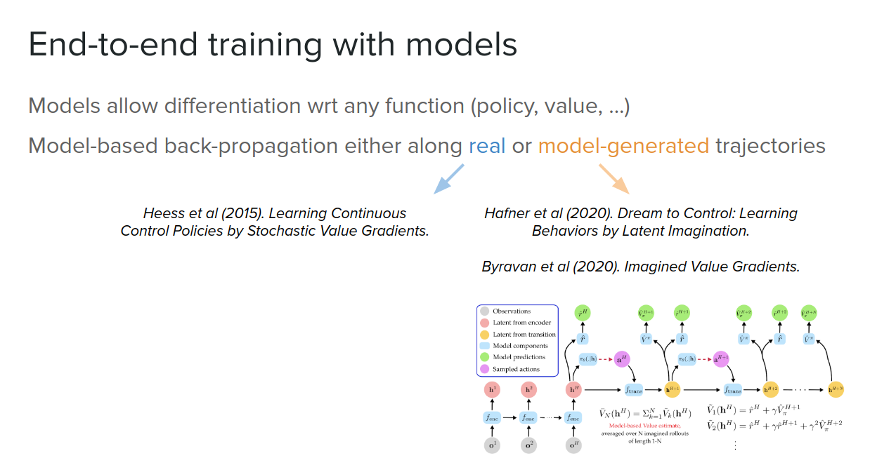
real trajectories are safer but need to be from the current policy parameters (so it’s less sample-efficient)
model-generated trajectories allow larger policy changes without interacting with the real world but might suffer more from model inaccuracies

Strengthening the policy

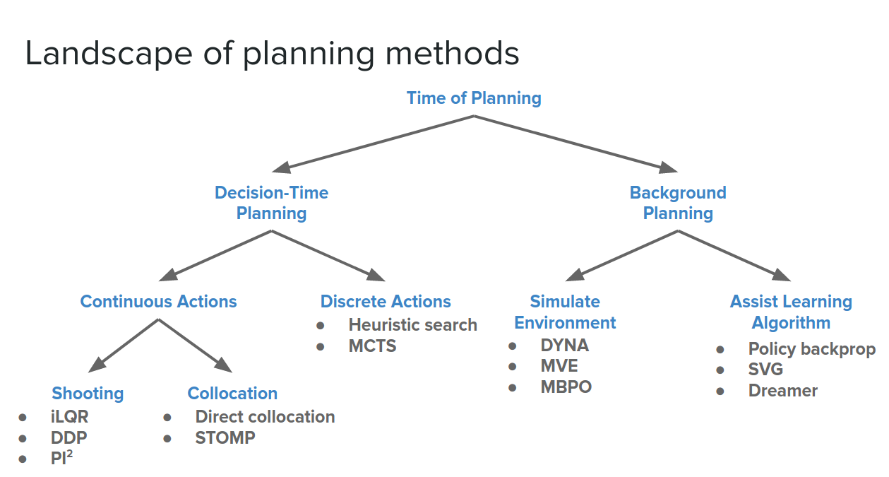
So far, we talked about the first two ways of using a model in RL. These two ways are in the category of Background Planning.

There is another category based on the Sutton and Barto (2018)- Reinforcement Learning: An Introduction categorization, called Decision-Time Planning, which is a unique option we have available in model-based settings.

What is the difference between background and decision-time planning?

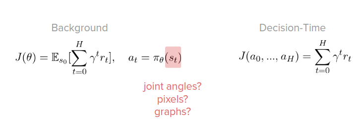
In background planning, we can think of it as answering the question, "how do I learn how to act in any possible situation to succeed and reach the goal?"

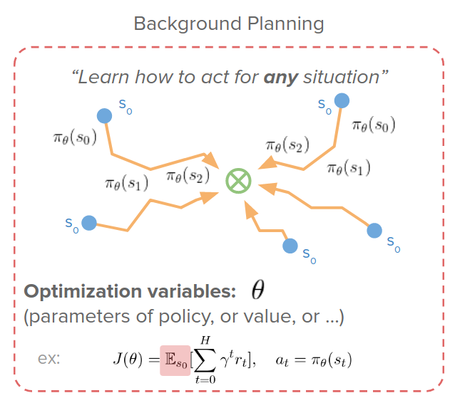
The optimization variables are parameters of a policy or value function or ..., and are trained using expectation over all possible situations.
Conceptually, we can think of background planning as learning a set of habits that we could reuse.
We can think of background planning as learning a fast type of thinking.

In decision-time planning, we want to answer the question, "what is the best sequence of actions just for my current situation to succeed or reach the goal?"

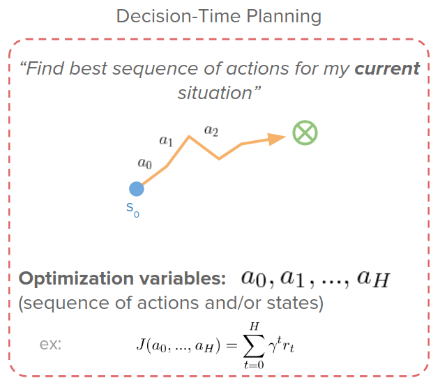
The optimization parameters are just a sequence of actions or states.
Conceptually, we can think of decision-time planning as finding our consciously improvising just for the particular situation that we find ourselves in.
We can think of decision-time planning as learning a slow type of thinking.

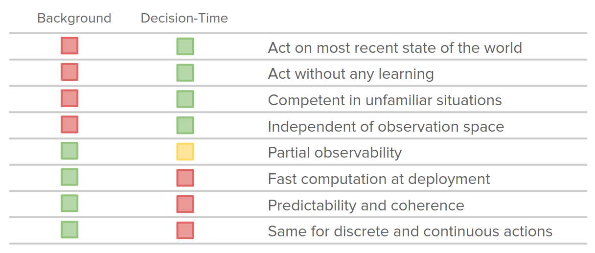
Why use one over the other?

Act on the most recent state of the world: decision-time planning is just concerned about the current state in finding the sequence of actions. You can act based on the most recent state of the world. By contrast, in background planning, the habits may be stale and might take a while to get updated as the world's changes.
Act without any learning: decision-time planning allows us to act without any learning at all. There is no need for policy or value networks before we can start making decisions. It is just an optimization problem as long as you have the model.
Competent in unfamiliar situations: if you find yourself in situations that are far away from where you were training, your set of habits or policy network might not have the competence (the ability to do something successfully or efficiently) there. So you don't have any information to act or are very uncertain, or even in the worst case, it will with confidence make decisions that just potentially make no sense. This is out of distribution and generalization problem. In these cases, decision-time planning would be more beneficial.
Independent of observation space: another advantage of decision-time planning is that it is also independent of the observation space that you decide on. In background methods, we need to consider some encoding or description of the state, joint angles, or pixels or graphs into our policy function. These decisions may play a large role in the total learning performance. When something is not working, you will not really know that is it because of the algorithm or state-space, which doesn't contain enough information. In contrast, decision-time planning avoids this confounded, which in practice can actually be quite useful when you're prototyping new methods.

Partial observability: decision-time plannings have some issues with it. They assume that you know the full state of the world when you're making the plan. So it's hard to hide information from decision-time planners. It is possible, but it is more costly.
Fast computation at deployment: decision-time planners require more computation. It is not just evaluating a habit, but it needs more thinking.
Predictability and coherence: decision-time planners do some actions which are not necessarily predictable or coherent. Because you are consciously thinking about each footstep, you might not have exactly the same plan. So you may have a very chaotic behavior that still succeeds. In contrast, background planning, because it learns a set of habits, it can perform a very regular behavior.
Same for discrete and continuous actions: background planning has a very unified treatment of discrete and continuous actions, which is conceptually simpler. In decision-time planning, there are different algorithms for discrete and continuous actions. We will see in the following sections more about them.

We can also mix and match the background and decision-time plannings.

What is the difference between discrete and continuous planning?

It depends on the problem which you want to solve. So it is not a choice that you can make. For example, in controlling a robot, the actions might be the torques for the motors (continuous), or in biomechanical settings, it might be muscle excitations (continuous), or in medical problems, the treatment that should be applied (discrete).

The distinction between discrete and continuous actions is not significant for background planning methods.

You just learn stochastic policies that sample either from discrete or continuous distributions.

$$ a \sim \pi(.|s) \quad \leftarrow Gaussian, categorical, ... $$

Backpropagation is still possible via some reparametrization techniques. See Jang et al (2016). Categorical reparametrization with Gumbel-Softmax for an example.

In either of these cases (continuous and discrete in background planning methods), your final objective and optimization problem is still smooth wrt the policy parameters because you are optimizing over expectations.

$$ J(\theta) = E_{\pi}[\sum_t r_t], \quad a_t \sim \pi(.|s_t, \theta) $$

But for decision-time planning, this distinction leads to specialized methods for discrete and continuous actions: discrete search or continuous trajectory optimization.

Let's see some examples to be able to compare them.

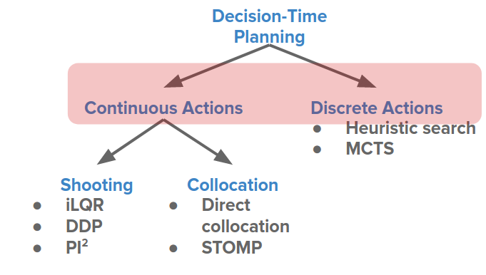
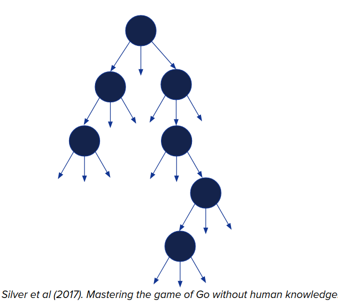
MCTS (monte carlo tree search)

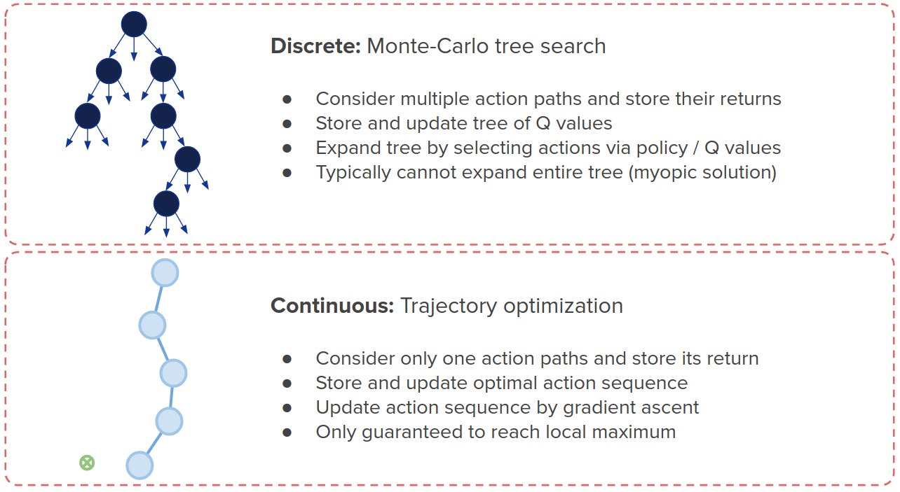
This algorithm is in a discrete action group and is used in alpha-go and alpha-zero. You keep track of Q-value, which is long term reward, for all states and actions that you want to consider. And also the number of times that the state and action have been previously visited.

Initialize $Q_0(s, a) = 0, N_0(s, a)=0, k=0$

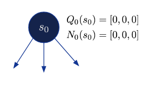
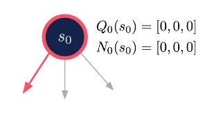
Expansion: Starting from the current situation and expand nodes and selecting actions according to a search policy:

$$\pi_k(s) = Q_k(s,a)$$

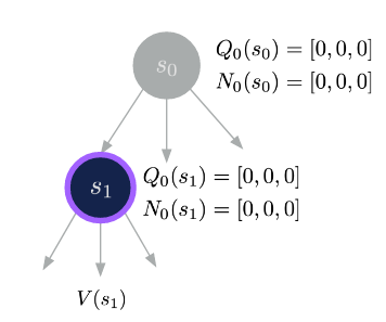
Evaluation: When a new node is reached, estimate its long-term value using Monte-Carlo rollouts

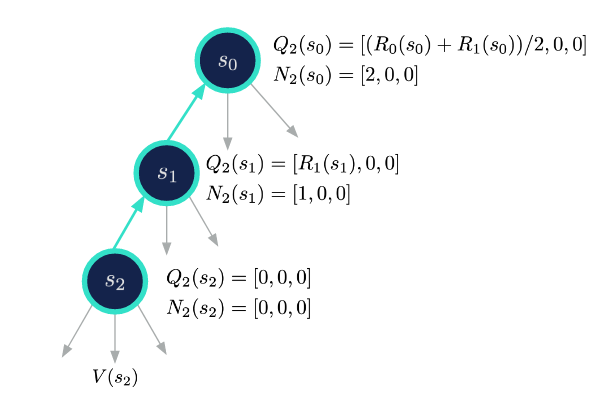
Backup: Propagate the Q-values to parent nodes:

$$ Q_{k+1}(s, a) = \frac{Q_k(s,a) N_k(s,a) + R}{N_k(s,a)+1} $$$$ N_{k+1}(s,a) = N_k(s,a)+1 $$

Repeat Steps 2-4 until the search budget is exhausted. $$ k = k + 1 $$

Trajectory Optimization

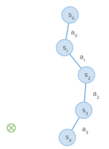
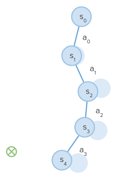
Instead of keeping track of a tree of many possibilities, you keep track of one possible action sequence.

Initialize $a_0, ..., a_H$ from guess

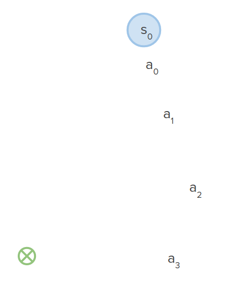
Expansion: execute sequence of actions $a = a_0, ..., a_H$ to get a sequence of states $s_1, ..., s_H$

Evaluation: get trajectory reward $J(a) = \sum_{t=0}^H r_t$
Back-propagation: because everything is differentiable, you can just calculate the gradient of the reward via back-propagation using reward model derivatives and transition model derivatives.

$$ \nabla_a J = \sum_{t=0}^H \nabla_a r_t $$$$ \nabla_a r_t = \nabla_s f_r(s_t, a_t) \nabla_a s_t + \nabla_a f_r (s_t, a_t) $$$$ \nabla_a s_t = \nabla_a f_s(s_{t-1}, a_{t-1}) + \nabla_s f_s(s_{t-1}, a_{t-1})\nabla_a s_{t-1} $$$$ \nabla_a s_{t-1} = ... $$

Update all actions via gradient ascent $ a \leftarrow a + \nabla_a J$ and repeat steps 2-5.

The differences between discrete and continuous actions can be summarized as follows:

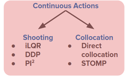
The continuous example we saw above can be categorized in shooting methods.

Variety and motivations of continuous planning methods

Why so many variations? They all try to mitigate the issues we looked at like:

Sensitivity and poor conditioning
Only reaches local optimum
Slow convergence

Addressing each leads to a different class of methods.

Sensitivity and poor conditioning

Shooting methods that we have seen have this particular issue that small changes in early actions lead to very large changes downstream.

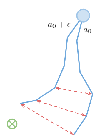
By expanding the objective function, this can be understood more clearly.

$$ \max_{a_0,...,a_H} \sum_{t=0}^H r(s_t, a_t), \quad s_{t+1} = f(s_t, a_t) $$$$ \sum_{t=0}^H r(s_t, a_t) = r(s_0, a_0) + r(f(s_0, a_0), a_1)+...+r(f(f(...),...), a_H) $$

It means that each state implicitly is dependent on all actions that came before it. This is similar to the exploding/vanishing gradient problem in RNNs that hurts long-term credit assignment. But unlike the RNN training, we cannot change the transition function because it is dictated to us by the environment.

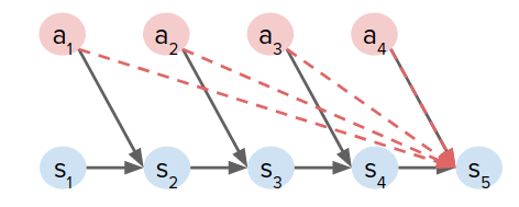
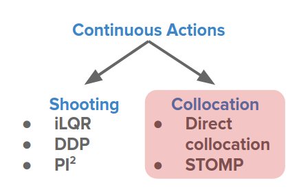
To address this problem, Collocation is introduced, which is optimizing for states and/or actions directly, instead of actions only. So we have a different set of parameters that we are optimizing over.

$$ \max_{s_0,a_0,...,s_H,a_H} \sum_{t=0}^H r(s_t, a_t), \quad ||s_{t+1} - f(s_t, a_t) || = 0 \leftarrow \text{explicit optimization constraint} $$

It is an explicit constrained optimization problem, rather than just beeng satisfied by construction as in shooting methods.

As a result, you only have pairwise dependencies between variables, unlike the dense activity graph in the previous figure for shooting methods.

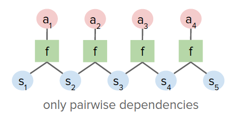
These methods have:

Good conditioning: changing $s_0, a_0$ has a similar effect as changing $s_H, a_H$.
Larger but easier to optimize search space. It is useful for contact-rich problems such as some robotics applications.

Only reaches local optimum

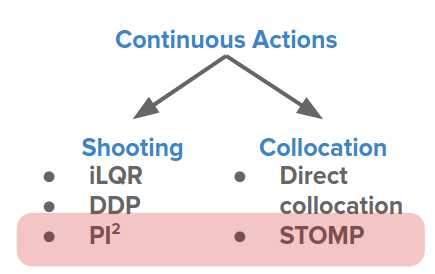
Some approaches try to avoid local optima like sampling-based methods: Cross-Entropy Methods (CEM) and $\text{PI}^2$.

For example, in CEMs, instead of just maintaining the optimal trajectory, it maintains the optimal trajectory's mean and covariance.

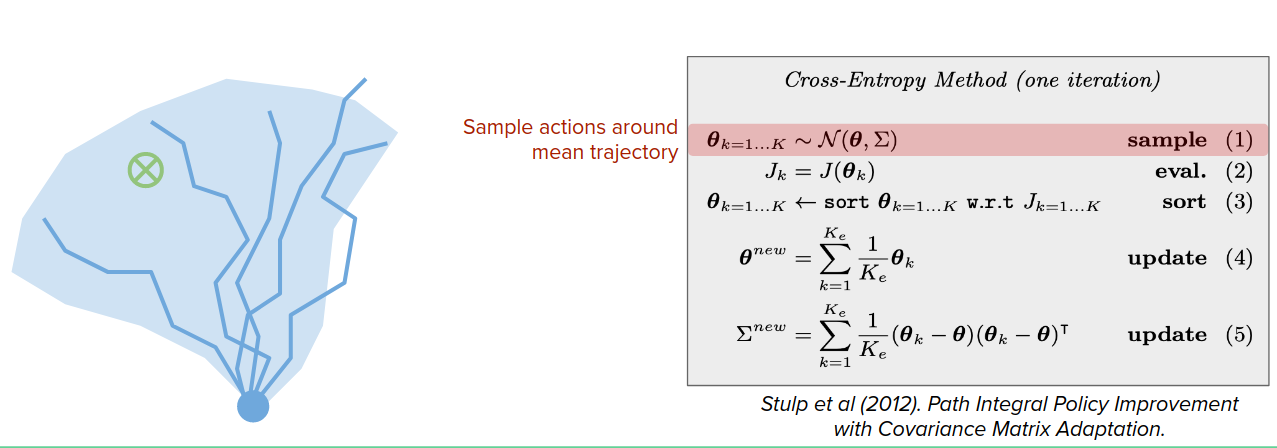
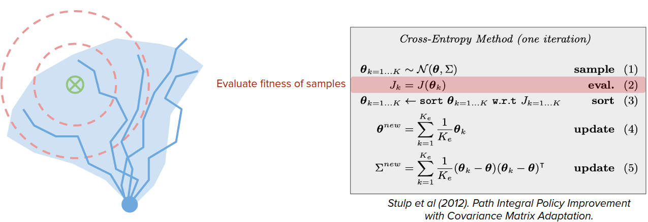
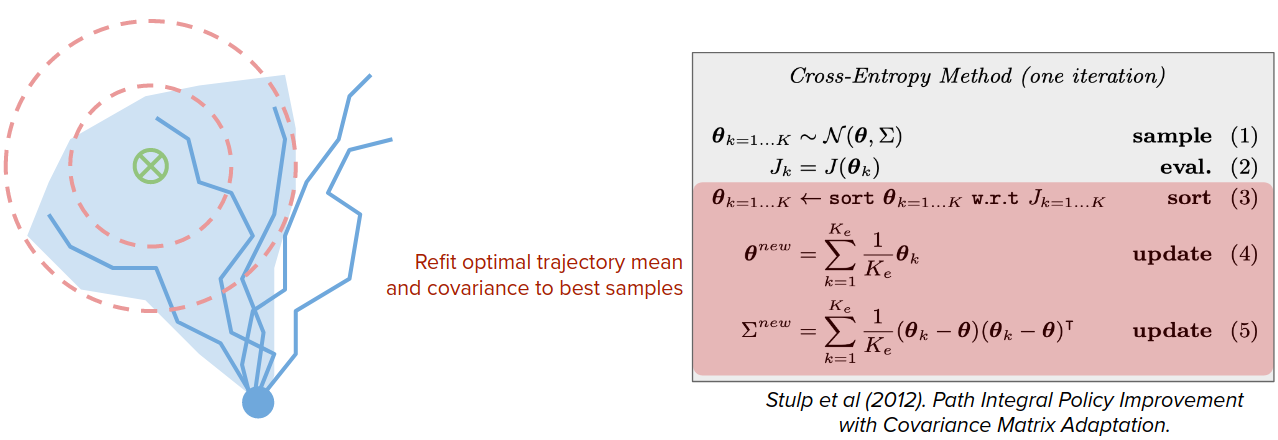
Despite being very simple, this works surprisingly well and has very nice guarantees on performance.

Why does this work?

Search space of decision-time plans much smaller than space of policy parameters: ex. 30x32 vs 32x644x32
More feasible plans than policy parameters

Slow convergence

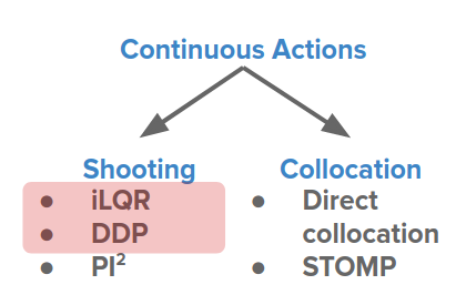
Gradient descent is too slow to converge, and we need to wait for thousands-millions of iterations to train a policy. But this is too long for a one-time plan that we want to through it away after.

Can we do something like Newton’s method for trajectory optimization, like non-linear optimization? YES!

We can approximate transitions with linear functions and rewards with quadratics:

$$ \max_{a_0,...,a_H} \sum_{t=0}^H r_t, \quad s_{t+1} = f_s(s_t, a_t), \quad r_t=f_r(s_t, a_t) $$$$ f_s(s_t, a_t) \approx As_t + Ba_t, \quad f_r(s_t, a_t) \approx s_t^TQs_t + a_t^TRa_t $$

Then it becomes the Linear-Quadratic Regulator (LQR) problem and can be solved exactly.

For iLQR, locally approximate the model around the current solution, solve the LQR problem to update the solution, and repeat.

For Differential dynamic programming (DDP), it is similar, but with a higher-order expansion of $f_s$.

Model-based control in the loop

We want to answer this question of how to both learn the model and act based on that simultaneously?

Gathering data to train models

How can we gather data to train the model? this is a chicken or the egg problem. Bad policy leads to a bad experience, leads to a bad model, leads to bad policy ...

This leads to some training stability issues in practice. There are some recent works in game theory to provide criteria for stability. See Rajeswaran et al (2020). A Game Theoretic Framework for Model Based Reinforcement Learning. for example.

Fixed off-line datasets

Another way to address this in the loop issues is to see if we can actually train from a fixed experience that is not related to the policy. Some options that we have are:

Human demonstration
Manually-engineered policy rollouts
Another (sub-optimal) policy

This leads to a recent popular topic model-based offline reinforcement learning. You can see some recent works like Kidambi et al (2020). MOReL: Model-Based Offline Reinforcement Learning., Yu et al (2020). MOPO: Model-based Offline Policy Optimization. See also: Levine et al (2020)., and Offline Reinforcement Learning: Tutorial, Review, and Perspectives on Open Problems.

Data augmentation

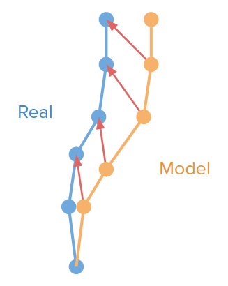
Another way to generate data is to use the model to generate data to train itself. For example, in Venkatraman et al (2014). Data as Demonstrator. You might have some trajectory of a real experiment that you got by taking certain actions; then you roll out the model and train to pull its predicted next states to true next states.

There are also some adversarial approaches to generate data to self-audit the model like Lin et al (2020). Model-based Adversarial Meta-Reinforcement Learning. and Du et al (2019). Model-Based Planning with Energy Models.

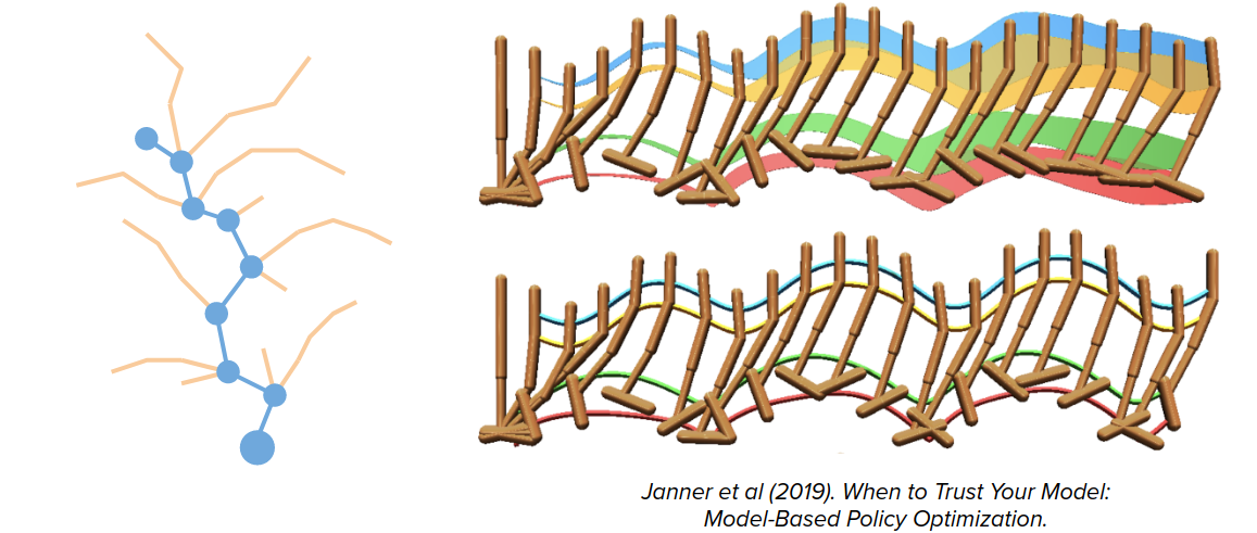
But even if we do all of these works, models are not going to be perfect. We cannot have experience everywhere, and there will be some approximation errors always. These small errors propagate and compound. We may end up in some states that are a little bit further away from true data, which might be an unfamiliar situation. So it might end up making even bigger errors next time around and so on and so forth that the model rollouts might actually land very far away over time from where you would expect them to be.

What's worse is that the planner might actually intentionally exploit these model errors to achieve the goal.

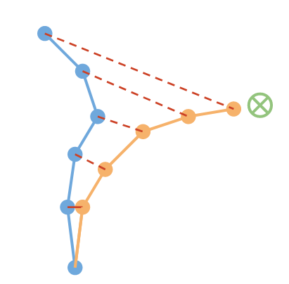
This leads to a longer model rollouts to be less reliable.

You can check Janner et al (2019). When to Trust Your Model: Model-Based Policy Optimization for more details.

Acting under imperfect models

The question is that "Can we still act with imperfect models?" the answer is yes!

Replan via model-predictive control

The first approach is to not commit to just one single plan (open-loop control) but continually re-plan as you go along (closed-loop control).

Let's see one example.

You might start at some initial state and create an imaginary plan using the trajectory optimization methods like CEM or other methods. Then apply just the first action of this plan. That might take you to some state that might not in the practice match with your model imagined you would end up with. But it's ok! You can just re-plan from this new state, again and again, take the first action and ... and by doing this, there is a good chance to end up near the goal.

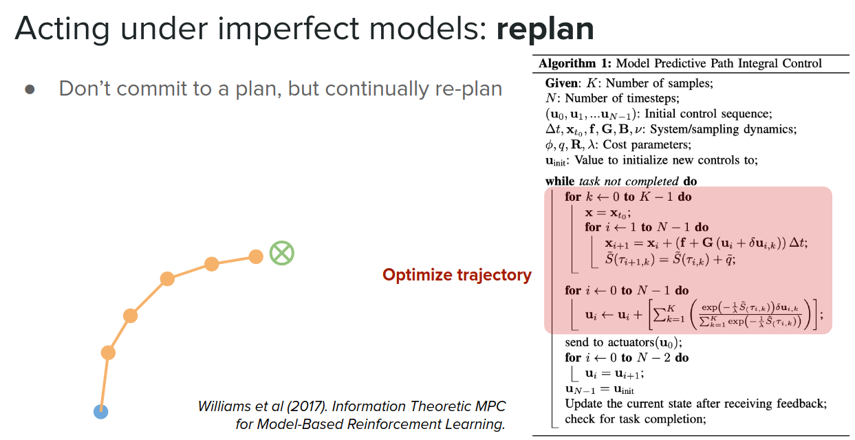
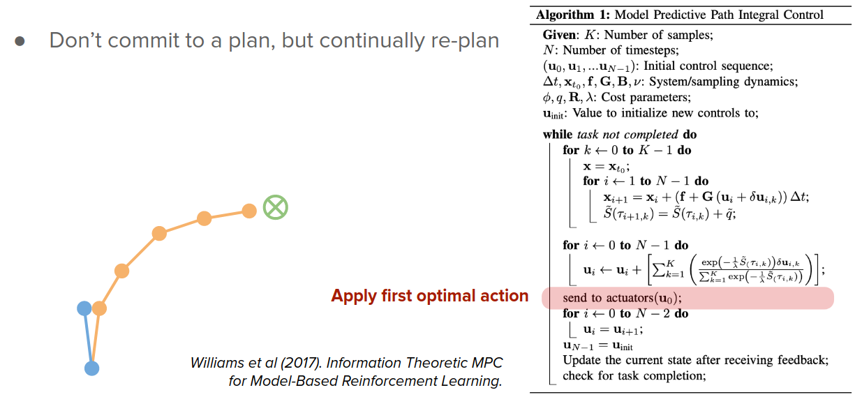
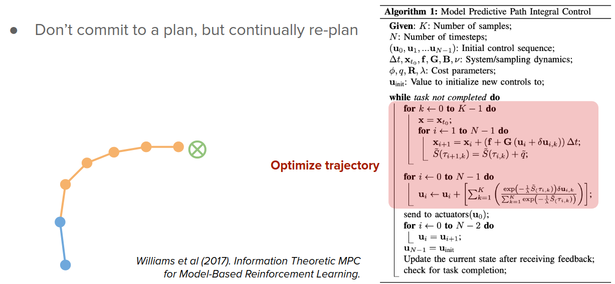
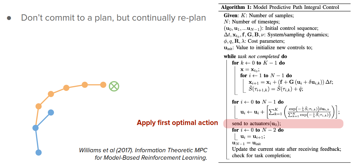
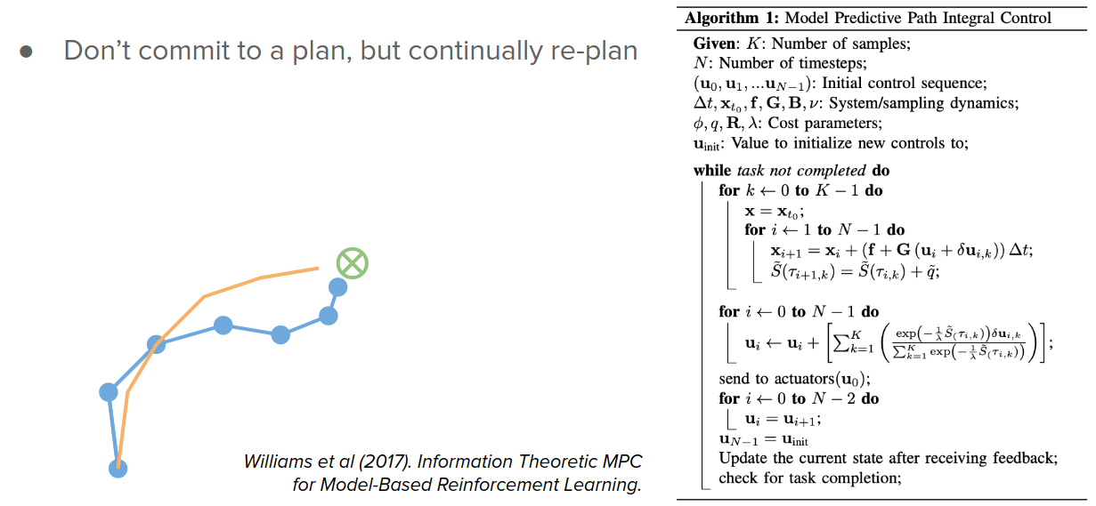
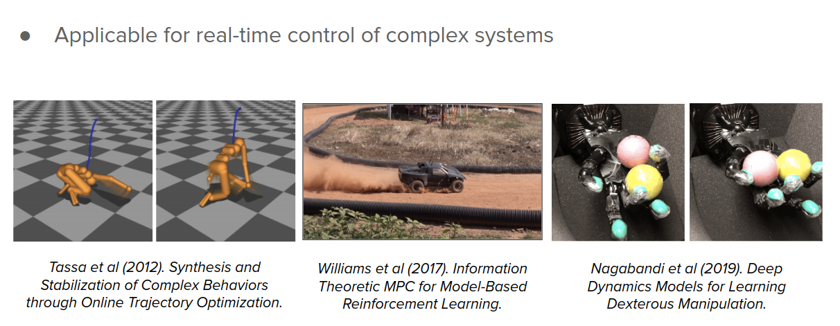
By doing this, the errors don't accumulate. So you don't need a perfect model; just one pointing in the right direction is enough. This re-planning might be expensive, but one solution is to reuse solutions from previous steps as initial guesses for the next plan.

Plan conservatively

We have'seen that longer rollouts become more unreliable. One solution would be just to keep the rollouts short. So we don't deviate too far from where we have real data. And as we saw in Dyna, just one single rollout can be also very helpful to improve learning.

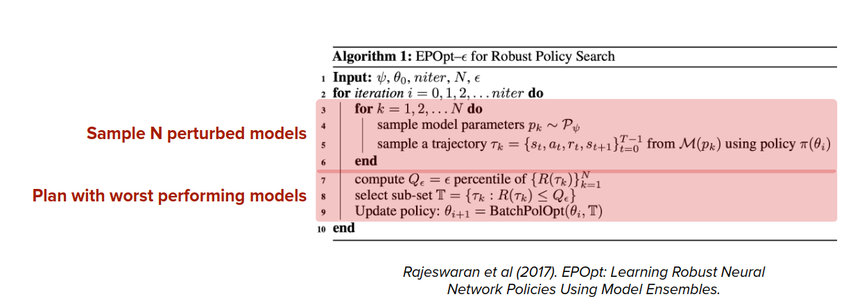
The other option to plan conservatively is to consider a distribution over your models and plan for either the average or worst case wrt distribution over your model or model uncertainty.

$$ \max_{\theta} E_{f \sim F} [\sum_t \gamma^t r_t], \quad a_t=\pi_{\theta}(s_t), \quad s_{t+1}=f_s(s_t, a_t), \quad r_t=f_r(s_t, a_t) $$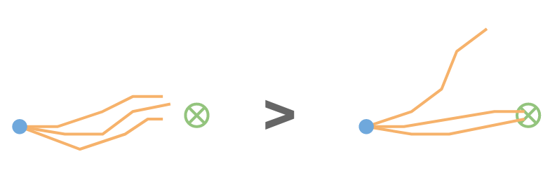

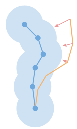
Another option for conservative planning is to try to stay close to states where the model is certain. There are a couple of ways to do this:

Implicitly: stay close to past policy that generated the real data
- Peters et al (2012). Relative Entropy Policy Search
- Levine et al (2014). Guided Policy Search under Unknown Dynamics.
Explicitly: add penalty to reward or cost function for going into unknown region
- Kidambi et al (2020). MOReL: Model-Based Offline Reinforcement Learning.

In the last two options for conservative planning, we need uncertainty. So how do we get this model uncertainty?

Estimating model uncertainty

Model uncertainty, if necessary for conservative planning, but it has other applications too that we will see later.

We consider two sources of uncertainty:

Epistemic uncertainty
- Model's lack of knowledge about the world
- Distribution over beliefs
- Reducible by gathering more experience about the world
- Changes with learning
Aleatoric uncertainty/Risk
- World's inherent stochasticity
- Distribution over outcomes
- Irreducible
- Static as we keep learning

There are multiple approaches to estimate these uncertainties, which are listed as follows:

Probabilistic neural networks that try to model distributions over the outputs of your model.
- Model explicitly outputs means and variances (typically Gaussian)
  
  $$ p(s_{t+1}|s_t, a_t) = N(\mu_{\theta}(s_t, a_t), \sigma_{\theta}(s_t, a_t))$$
- Simple and reliable (supervised learning)
- Only captures aleatoric uncertainty/risk
- No guarantees for reasonable outputs outside of training data

Bayesian neural network
- Model has a distribution over neural network weights
  
  $$ p(s_{t+1}|s_t, a_t) = E_{\theta}[p(s_{t+1}|s_t, a_t, \theta)]$$
- Captures epistemic and aleatoric uncertainty
- Factorized approximations can underestimate uncertainty
- Can be hard to train (but an active research area)

Gaussian processes
- Captures epistemic uncertainty
- Explicitly control state distance metric
- Can be hard to scale (but an active research area)
Pseudo-counts
- Count or hash states you already visited
- Captures epistemic uncertainty
- Can be sensitive to state space in which you count

Ensembles
- Train multiple models independently and combine predictions across models
- Captures epistemic uncertainty
- Simple to implement and applicable in many contexts
- Can be sensitive to state space and network architecture

For discussion in the context of reinforcement learning, see Osband et al (2018). Randomized Prior Functions for Deep Reinforcement Learning.

Between the above options, Ensembles are currently popular due to simplicity and flexibility.

Combining planning and learning

We compared these two methods in previous sections and saw that background and decision-time planning have complementary strengths and weaknesses.

How to combine decision-time planning and background planning methods and get the benefits of both?

Distillation

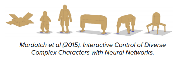
In this approach, we gather a collection of initial states and run our decision-time planner for each initial state and get a collection of trajectories that succeed at reaching the goal. Once we collected this collection of optimal trajectories, we can use a supervised learning algorithm to train either policy function or any other function to map states to actions. This is similar to Behavioral Cloning (BC).

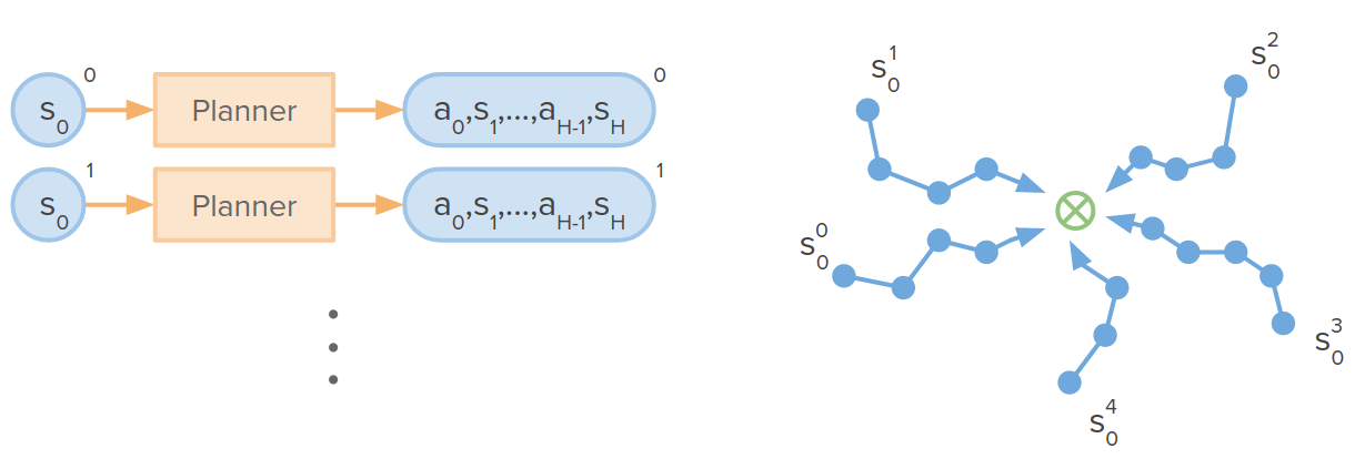
Some issues that can arise:

What is the learned policies that have compounding errors? If we rollout the policy from one of the states, it does something different than what we intended to do.

Create new decision-time plans from these states that have been visited by the policy.
Add these trajectories (new decision-time plans) to the distillation dataset (expand dataset where policy makes errors)

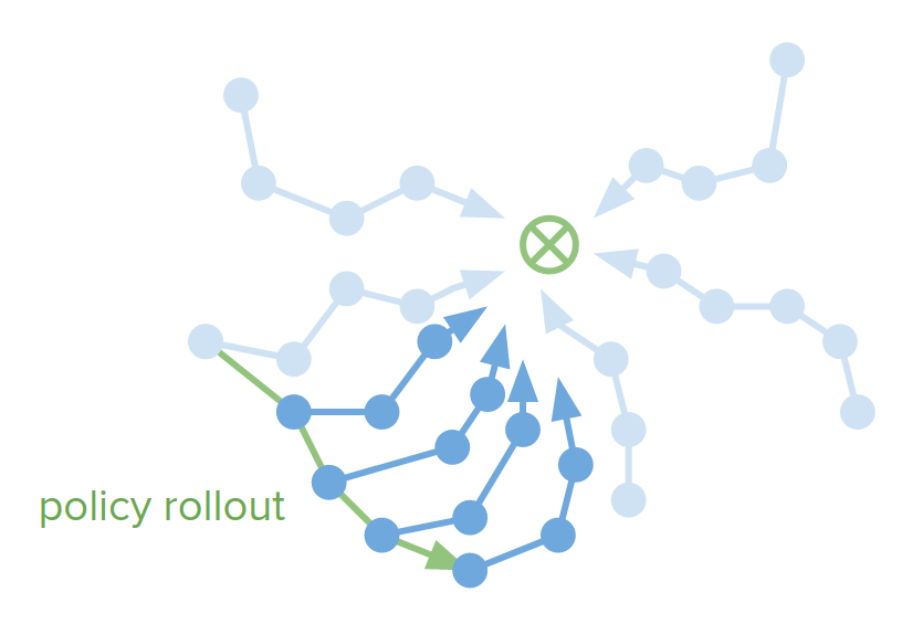
This is the idea of Dagger algorithm:

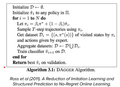
What if the plans are not consistent? There are several ways to achieving a goal, and we've seen that by changing the initial condition only a little bit, the decision-time planner can give us pretty different solutions to reach a single goal. This chaotic behavior might be hard to distill into the policy

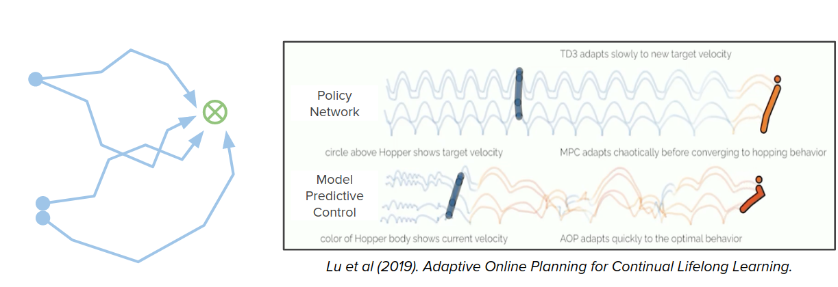
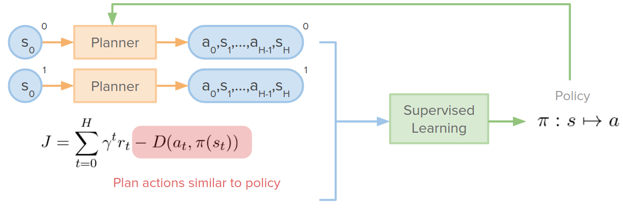
we can make it so that the policy function that we are learning actually feeds back and influences our planner.
To do this, we can add an additional term in our cost that says stay close to the policy. $D$ in the below cost function is the distance between actions of the planner, $a_t$, and the policy outputs, $\pi(s_t)$.

Terminal value functions (value of the terminal state)

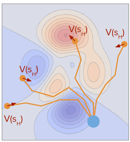
One of the issues with many trajectory optimizations or discrete search approaches is that the planning horizon is typically finite. This may lead to myopic or greedy behavior.

$$ J^H = \sum_{t=0}^H \gamma^t r_t $$

To solve this problem, we can use the value function at the terminal state and add it to the objective function. This learned value function guides plans to good long-term states. So the objective function would be infinite horizon:

$$ J^{\infty} = \sum_{t=0}^{\infty} \gamma^t r_t = \sum_{t=0}^H \gamma^t r_t + \gamma^H V(s_H) $$

This is another kind of combining decision-time planning (optimization problem) with background planning (learned value function).

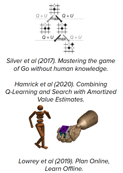
This can be used in both discrete and continuous action spaces:

Planning as policy improvement

So far, we used policy (background) or decision-time planner to make a decision and generate trajectory and actions.

But we can combine them and use the planner as policy improvement. We can use the policy to provide some information for the planner. For example, the policy can output its set of trajectories, and the planner can use it as a warm start or initialization to improve upon. We would like to train the policy such that the improvement proposed by the planner has no effect. So the policy trajectory is the best that we can do. I think we can see the planner as a teacher for the policy.

Some related papers are listed here:

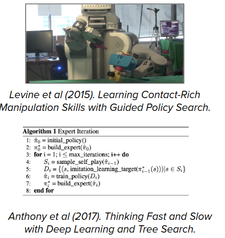
Silver et al (2017). Mastering the game of Go without human knowledge.
Levine et al (2014). Guided Policy Search under Unknown Dynamics.
Anthony et al (2017). Thinking Fast and Slow with Deep Learning and Tree Search.

Implicit planning

In addition, to use a planner to improve policy trajectory, we can put the planner as a component inside the policy network and train end-to-end.

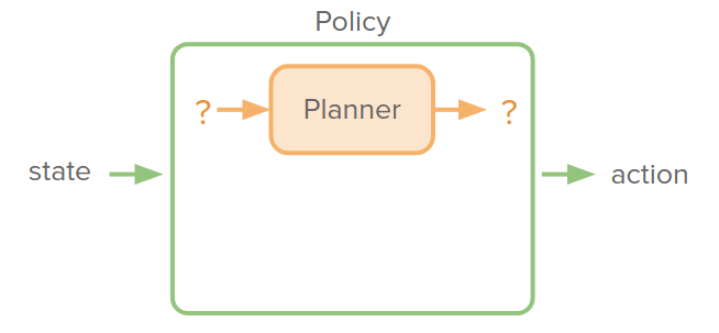
The advantage of doing this is that the policy network dictates abstract state/action spaces to plan in. But the downside of this is that it requires differentiating through the planning algorithm. But the good news is that multiple algorithms we've seen have been made differentiable and amenable to integrating into such a planner.

some examples are as follows:

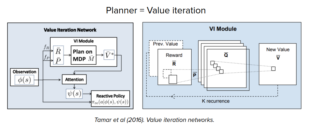
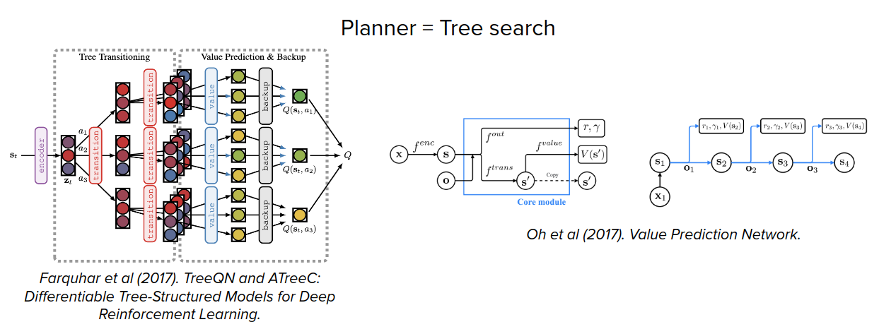
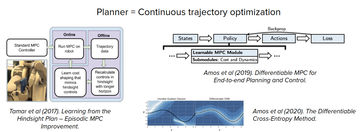
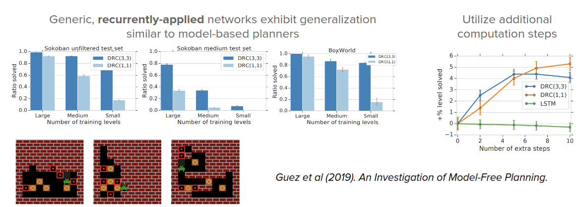
There are also some works that show the planning could emerge in generic black-box policy network and model-free RL training.

What else can models be used for?

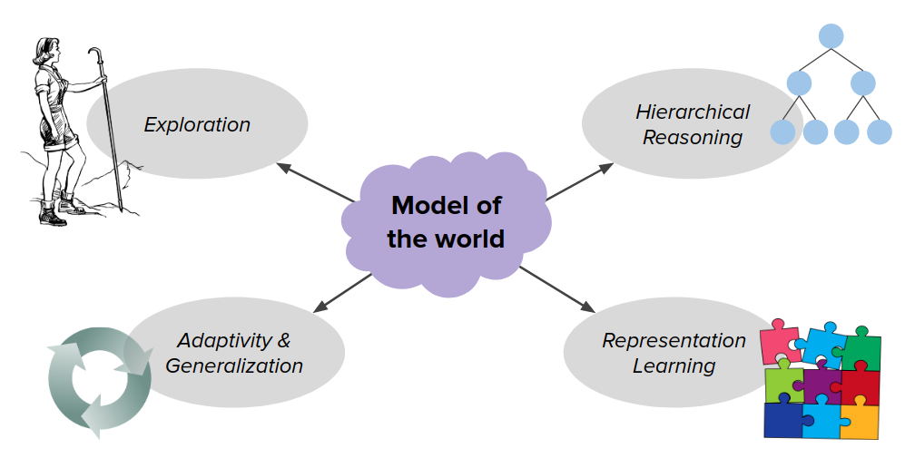
Consider we have a model of the world. We can use the model in a lot of different ways like:

Exploration
Hierarchical Reasoning
Adaptivity & Generalization
Representation Learning
Reasoning about other agents
Dealing with partial observability
Language understanding
Commonsense reasoning
and more!

Here we're gonna just focus on the first four ways that we can use the model to encourage better behavior.

Exploration

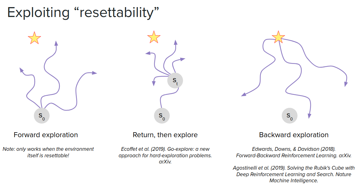
One of the good things about having a model of the world is that you can reset to any state in the world that you might care about. It's not possible in all environments to reset like a continual learning problem. But if you have the model of the world, you can reset to any state you want.

We can also consider resetting to intermediate states in the middle of the episode as a starting point. The idea is to keep track of one of the interesting states and does exploration from there. So if you have the world's model, you can again reset to that state and efficiently perform additional explorations.

You can also reset from the final state rather than the initial state. This can be useful in situations where there is only a single goal state like Rubik's Cube. In this case, there is only one goal but maybe several possible starting states. So it would be useful to reset to the final state and explore backward from there rather than starting from the initial state.

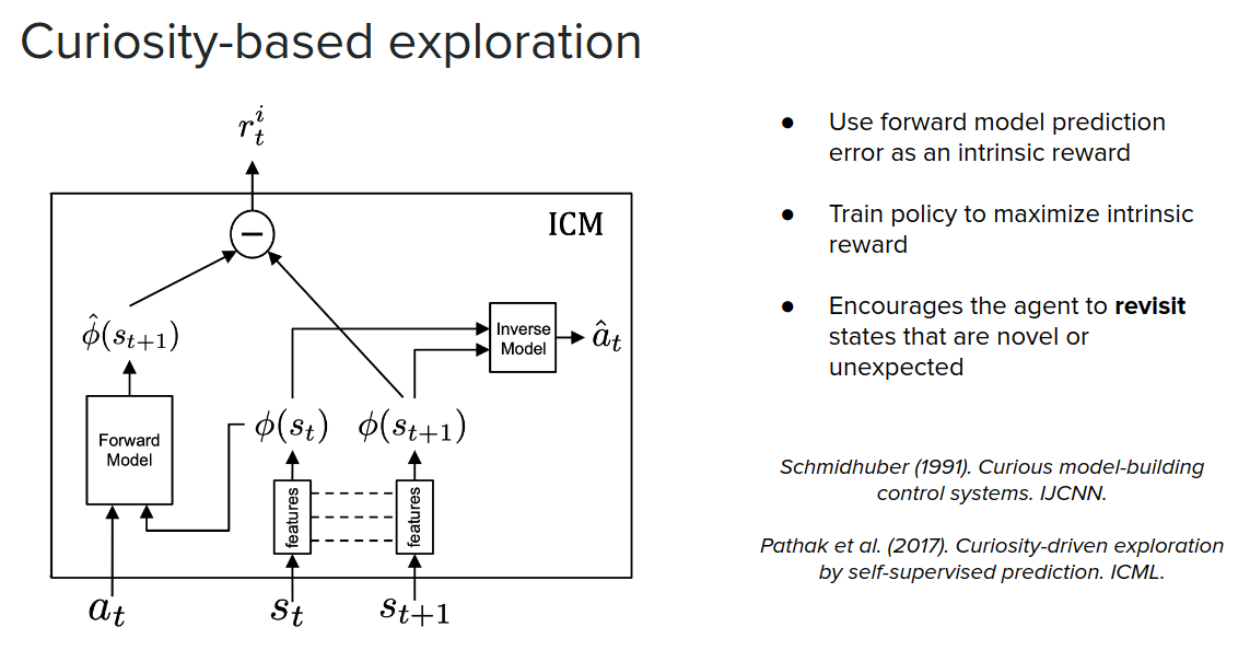
Another way that models can be used to facilitate exploration is by using intrinsic reward. In these cases, we want to explore places that we haven't been much so that we can gather data in those locations and learn more about them. One way to identify where we haven't been is to use model prediction error as a proxy. Basically, we learn a world model, then we predict what the next state is going to be and then take action and observe the next state and compare it with the predicted state and calculate the model error. We can then use this prediction error as a signal in the intrinsic reward to encourage the agent to explore the locations we haven't visited often to learn more about them.

In addition to the above approach, we can also plan to explore. In POLO paper, rather than using the error from your prediction model, they use the error across an ensemble of value functions and use it as an intrinsic reward. Actually, at each state, we compute a bunch of different values from our ensemble of value functions, then take softmax over them to give us an optimistic estimate of what the value is going to be. We can use this optimistic value estimate as an intrinsic reward. We plan to maximize this optimistic value estimate, and then this allows us to basically, during planning, identify places that we should direct our behavior towards are more surprising or more interesting.

Compute intrinsic reward during (decision-time) planning to direct the agent into new regions of state-space
Intrinsic reward = softmax across an ensemble of value functions

$$ \hat{V}(s) = log(\sum_{k=1}^K exp(k\hat{V}_{\theta_k}(s))) $$

Lowrey et al. (2019). Plan Online, Learn Offline: Efficient Learning and Exploration via Model-Based Control. ICLR 2019.

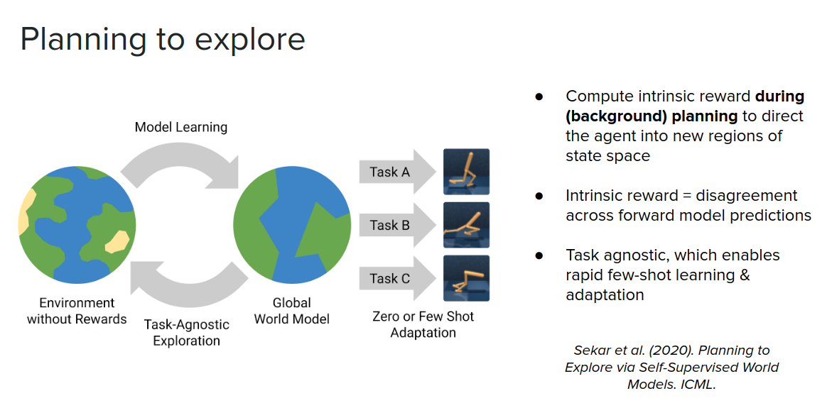
We can also use the same idea, but instead of using a set of disagreement across on ensemble of value functions, we can compute disagreement across transition functions. Now because we are just using state transitions, this turns into a task agnostic exploration problem. We can then plan where there is a disagreement between our transition functions and direct behavior towards those regions of space to learn a really robust world model. And then use this model of the world to learn new tasks either using zero-shot or few-shot (examples of experience).

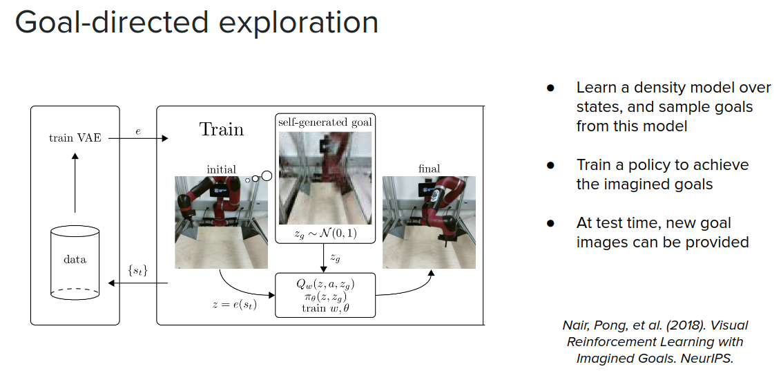
Finally, another form of exploration is that if we have a model of possible states that we might find ourselves in, not necessarily a transition model but a density model over goals, we can sample possible goals from this density model and then train our agent achieve the goals.

Hierarchical reasoning

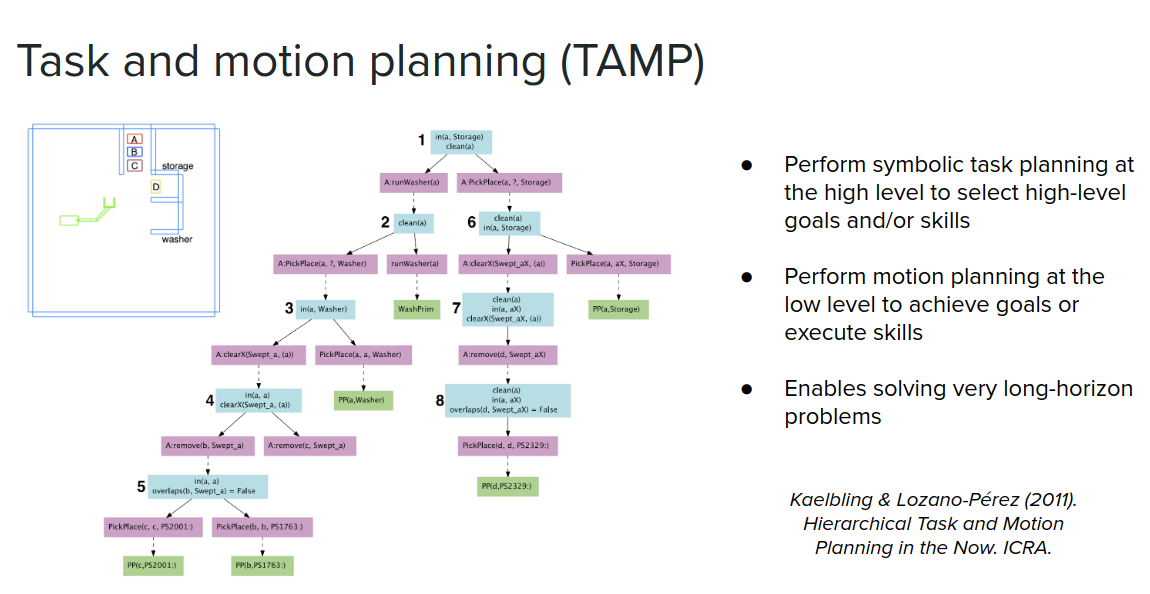
A very classic way of doing hierarchical reasoning is what's called task and motion planning (TAMP) in robotics. You jointly plan symbolically at the task level, and then you also plan in the continuous space and do motion planning at the low-level—you sort of doing these things jointly in order to solve relatively long-horizon and multi-step tasks. For example, in the following figure, to control a robot arm and to get block $A$ and put it in the washer, wash it, and then put it in storage. In order to do this, you first have to move $C$ and $B$ out of the way and put $A$ into the washer, then move $D$ out of the way and then put $A$ into the storage. By leveraging symbolic representation, like PDDL from the beginning of the post, allows you to be able to jointly solve these hierarchical tasks.

The other example of this is the OpenAI Rubik's Cube solver. The idea is that you use a high-level symbolic algorithm, Kociemba's algorithm, to generate the solution (plan) of high-level actions, for example, which faces should be rotated, and then you have a low-level neural network policy that generates the controls needed to achieve these high-level actions. This low-level control policy is quite challenging to learn.

OpenAI et al. (2019). Solving Rubik's Cube with a Robot Hand. arXiv.

The question that might arise is that where does this high-level state-space come from?

We don't want to hand-code symbolically on these high-level roles that we want to achieve. Some model-free works try to answer this, but we focus on some MBRL approaches here for this problem.

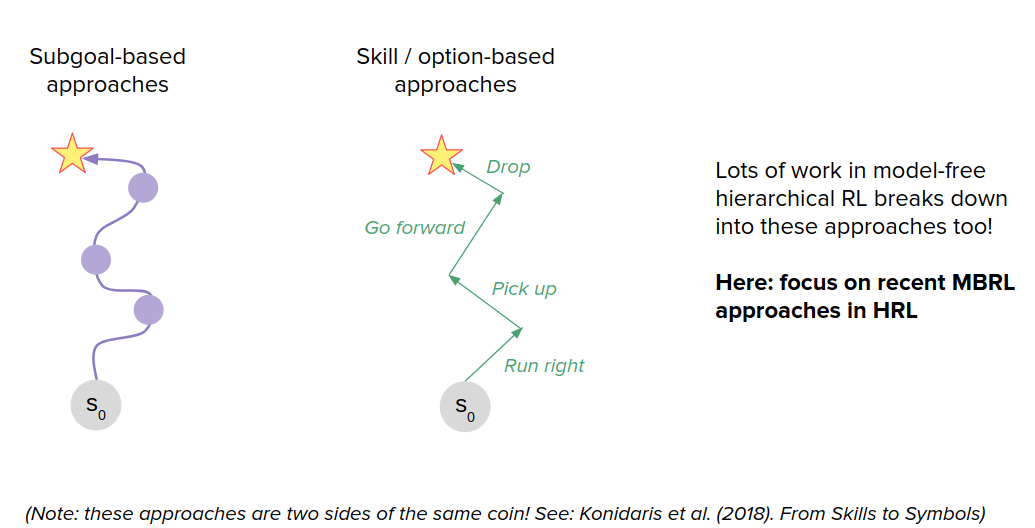
Subgoal-based approaches

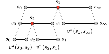
We can consider that any state you might find yourself in in the world as a subgoal. We don't want to construct a super long sequence of states to go through, but a small sequence. So the idea would be which states do we pick as a subgoal. Rather than learning a forward state transition model, we can learn a universal value function approximator, $V(s, g)$, that tells us the value of going from state $s$ to goal state $g$. We can train these value functions between our subgoals to estimate how good a particular plan of length $k$ is. A plan of length $k$ is then given by maximizing:

$$ \text{arg}\max_{\{s_i\}_{i=1}^k} (V(s_0, s_1) + V(s_k, s_g) + \sum_{i=1}^{k-1} V(s_i, s_{i+1})) $$

The figure below shows the idea. If you start from state $s_0$ and you want to go to $s_{\infty}$, you can break up this long plan of length one into a plan of length two by inserting a subgoal. You can do this recursively multiple times to end up with a plan of length $k$ or, in this case, a plan of length three.

When we use a planner to identify which of these subgoals we should choose in order to maximize the above equation, in the figure below, you see which white subgoal it is considering as subgoal in order to find a path between the green and the blue points.

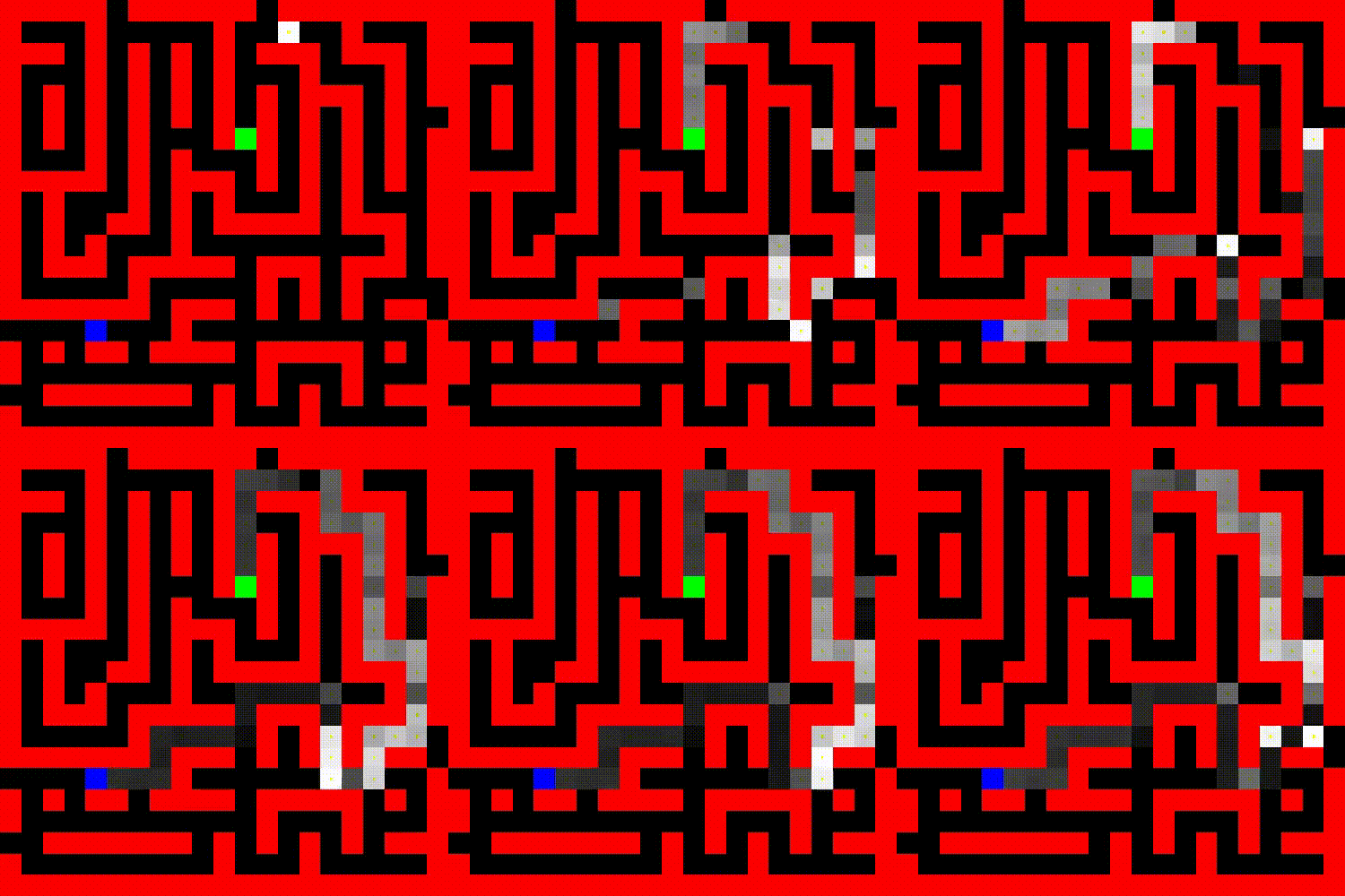
Nasiriany et al. (2019). Planning with Goal-Conditioned Policies. NeurIPS.
Jurgenson et al. (2019). Sub-Goal Trees -- A Framework for Goal-Directed Trajectory Prediction and Optimization. arXiv.
Parascandolo, Buesing, et al. (2020). Divide-and-Conquer Monte Carlo Tree Search For Goal-Directed Planning. arXiv.

Skill-based approaches

Here, rather than identifying discrete states as subgoals that we want to try to achieve, what we want to do is to learn a set of skills that sort of fully parametrize the space of possible trajectories that we might want to execute. So, for example, in the Ant environment, a nice parametrization of skills would be to say a particular direction that you want to get to move in. So the approach taken by this paper is to learn a set of skills those outcomes are both (1) easy to predict, so if you train a dynamics model to predict the outcome of executing the skill, and (2) the skills are diverse from one another. That's why you get this nice diversity of the ant moving in different directions. This works very well for zero-shot adaptation to new sequences of goals. As you can see on the bottom, this is an ant going to a few different locations in space, and it is doing this by just pure planning using this set of skills that it is learned during the unsupervised training phase.

Learn a set of skills whose outcomes are (1) easy to predict and (2) diverse
Learn dynamics model over skills, and plan with MPC
Can solve long-horizon sequences of high-level goals with no additional learning

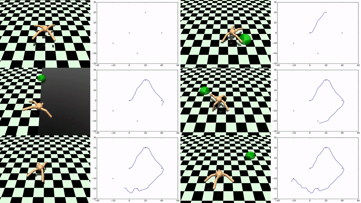
Sharma et al. (2020). Dynamics-Aware Unsupervised Discovery of Skills. ICLR.

representation Learning

Beyond just using models for prediction, they can be used as regularizers for training other types of representations that then you can train a policy on.

One way is to learn a model as an auxiliary loss. For example, if you have an A2C algorithm and add an auxiliary loss to predict the reward it's gonna achieve, in some cases, you can get a large improvement in performance by just adding this auxiliary loss. By considering this loss during training, we are actually forcing it to learn the future and capture the structure of the world, which is useful. We also don't use this learned model in planning and just for representation learning.

Jaderberg et al. (2017). Reinforcement learning with unsupervised auxiliary tasks. ICLR 2017.

The other same idea is to use a contrastive loss, like CPC paper (below), that tries to predict what observations it might encounter in the future, and by adding this additional loss during training, we see improvement in performance.

van den Oord, Li, & Vinyals (2019). Representation Learning with Contrastive Predictive Coding. arXiv.

Another idea is plannable representations that make it much easier to plan in. For example, if we are in a continuous space, we can discretize it in an intelligent way that might make it easy to use some of these discrete search methods, like MCTS, to rapidly come up with a good plan of actions. Or maybe we can come up with a representation for our state space such that moving along a direction in the latent state space corresponds to planning. So you can basically just interpolate between states in order to come up with a plan.

Learn an embedding of states that is easier to plan in, e.g.
- Discretized
- States that can be transitioned between should be near to each other in latent space!
Related to notions in hierarchical RL (state abstraction)

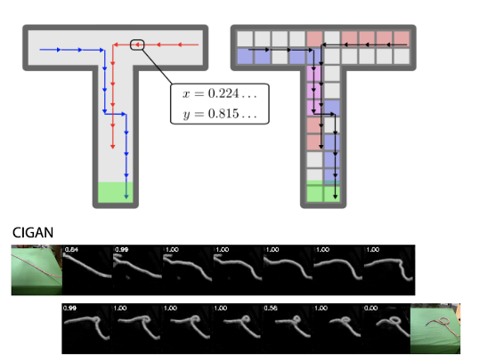
Corneil et al. (2018). Efficient Model-Based Deep Reinforcement Learning with Variational State Tabulation. ICML.
Kurutach et al. (2018). Learning Plannable Representations with Causal InfoGAN. NeurIPS.

Adaptivity & generalization

Models of the world can also be used for fast adaptation and generalization.

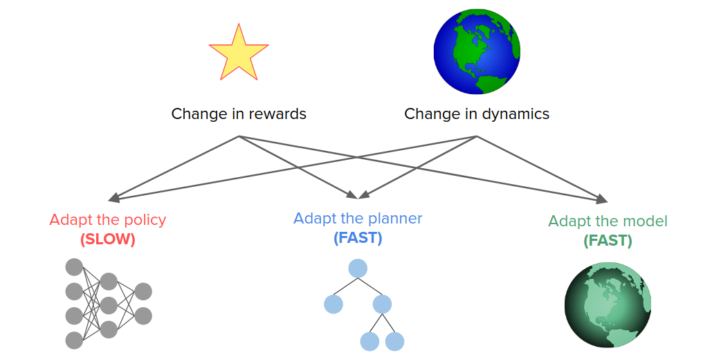
The world can be changed in two different ways:

Change in rewards. So we're being asked to do a new task, but the dynamics are the same.
Change in dynamics.

Based on the above changes, we can do different things in response to them.

In a model-free approach, we just adapt to the policy. But this tends to be relatively slow because it's hard to quickly adapt changes in rewards to the same dynamics and vice versa because they are sort of entangled with each other.

If we have an explicit model of the world, we can update our behavior differently. One option would be that we can adapt the planner, but we can also adapt the model itself, or we can do both.

Adapting the planner in new states

A pre-trained policy may not generalize to all states (especially in combinatorial spaces). So some states that we might find ourselves in might be required harder or more reasoning, and others may require less. We have to try to detect when planning is required, and they adapt the amount of planning depending on the difficulty of the task. For example, in the following gifs, in the upper case, the n-body agent can easily solve the task and reach the center's goal using just a couple of simulations. But in the bottom case, it is much harder to reason about because it starts on one of the planets, which requires many more simulations. We can adaptively change this amount of computation as needed. Save the computation on easy scenes and then spend it more on the hard ones.

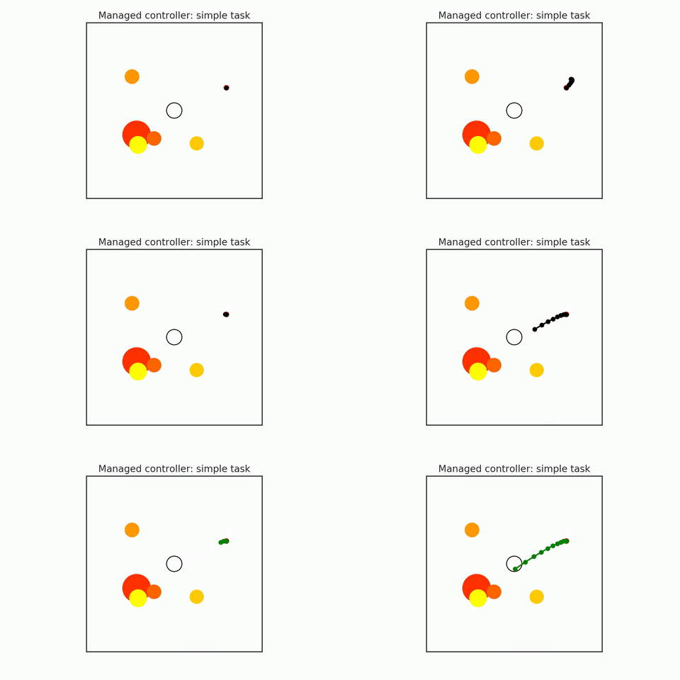
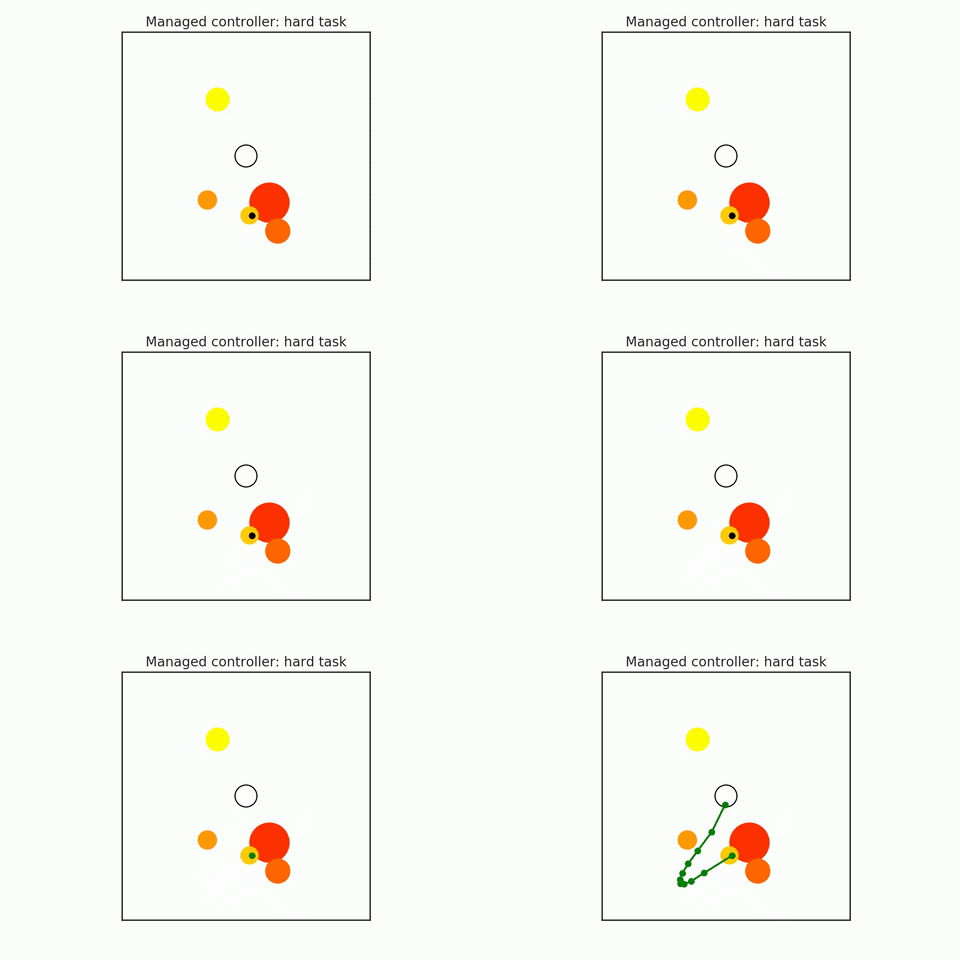
Hamrick et al. (2017). Metacontrol for adaptive imagination-based optimization. ICLR 2017.
Pascanu, Li, et al. (2017). Learning model-based planning from scratch. arXiv.

Adapting the planner to new rewards

Here is another same idea in a life-long learning setup where the reward can suddenly change, and either the agents can observe the change in the reward, or they just have to infer the reward has changed. Because of changes in reward, it needs more planning because the prior policy is less reliable, and more planning allows you to better explore these different options for the reward function. In the video below, as you can see in the bottom agent after the reward is changed, the agent needs to do more planning to have a nice movement compared to the other two agents.

Lu, Mordatch, & Abbeel (2019). Adaptive Online Planning for Continual Lifelong Learning. NeurIPS Deep RL Workshop.

Adapting the model to new dynamics

For the times that the dynamics change, it could be very useful to adapt the model. One way to approach this is to train the model using the meta-learning objective so that during training, you're always training it to adapt to a slightly different environment around you, and at the test time, you actually see a new unobserved environment that you never saw before, you can take a few gradient steps to adapt the model to deal with these new situations. Here is an example where the agent, half cheetah, has been trained to walk along some terrain, but it's never seen as a little hill before. Therefore, the baseline methods that cannot adapt their model cannot get the agent to go up the hill, where this meta-learning version can get the cheetah to go up the hill.

Nagabandi et al. (2019). Learning to Adapt in Dynamic, Real-World Environments through Meta-Reinforcement Learning. ICLR.

What's missing from model-based methods?

Humans are ultimate model-based reasoners and we can learn a lot from how we build and deploy models of the world. - Motor control: forward kinematics models in the cerebellum. We have a lot of motor systems that are making predictions about how our muscles are going to affect the kinematics of our bodies.

Language comprehension: we build models of what is being communicated in order to understand.
Pragmatics: we construct models of listener & speaker beliefs in order to try to understand what is tryingto be communicated.
Theory of mind: we construct models of other agents’ beliefs and behavior in order to predict what they are going to do.
Decision making: model-based reinforcement learning
Intuitive physics: forward models of physical dynamics
Scientific reasoning: mental models of scientific phenomena
Creativity: being able to imagine novel combinations of things
… and much more!

For more you can see the following reference:

Markman, Klein, & Suhr (2008). Handbook of Imagination and Mental Simulation.
Abraham (2020). The Cambridge Handbook of the Imagination.

If you look at the mentioned different domains, where people are engaging a model based reasoning, a few themes emerge that could be really useful in thinking about how to continue to develop our models in MBRL.

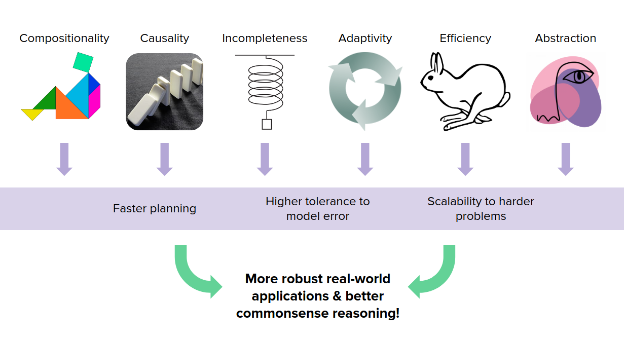
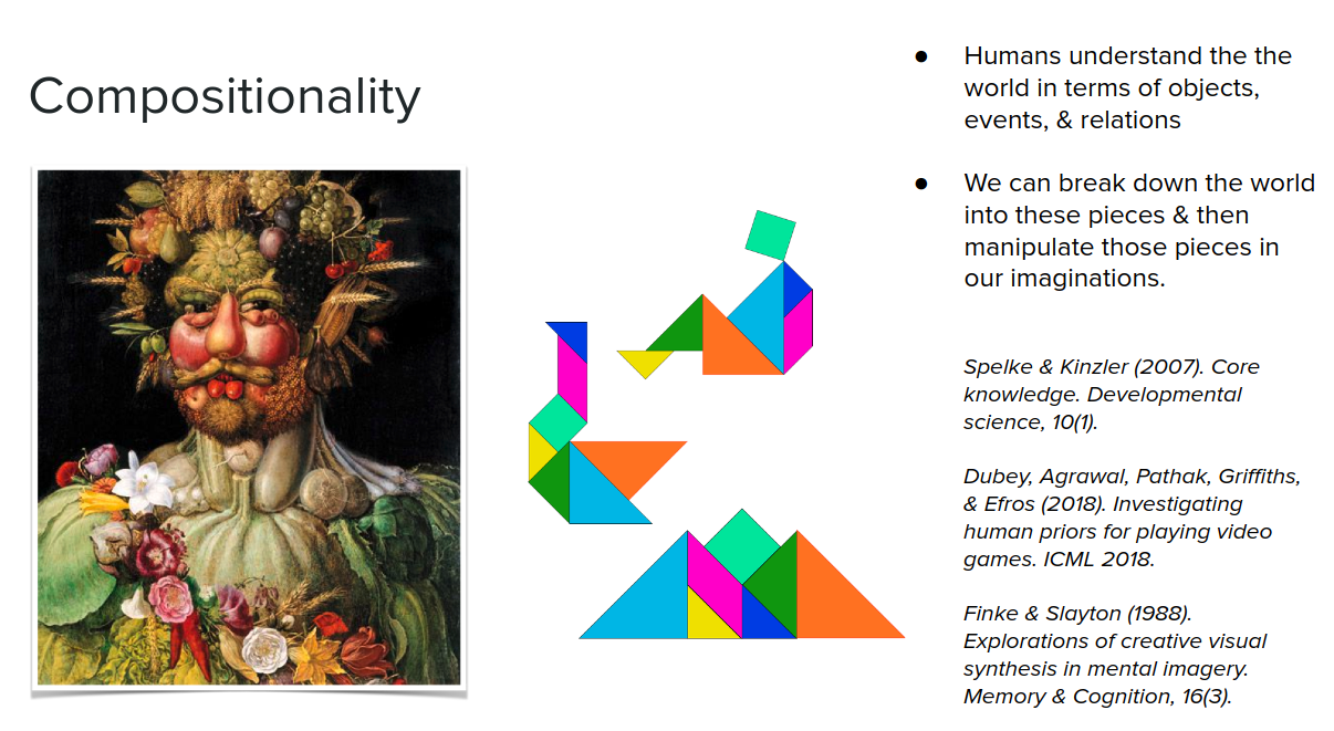
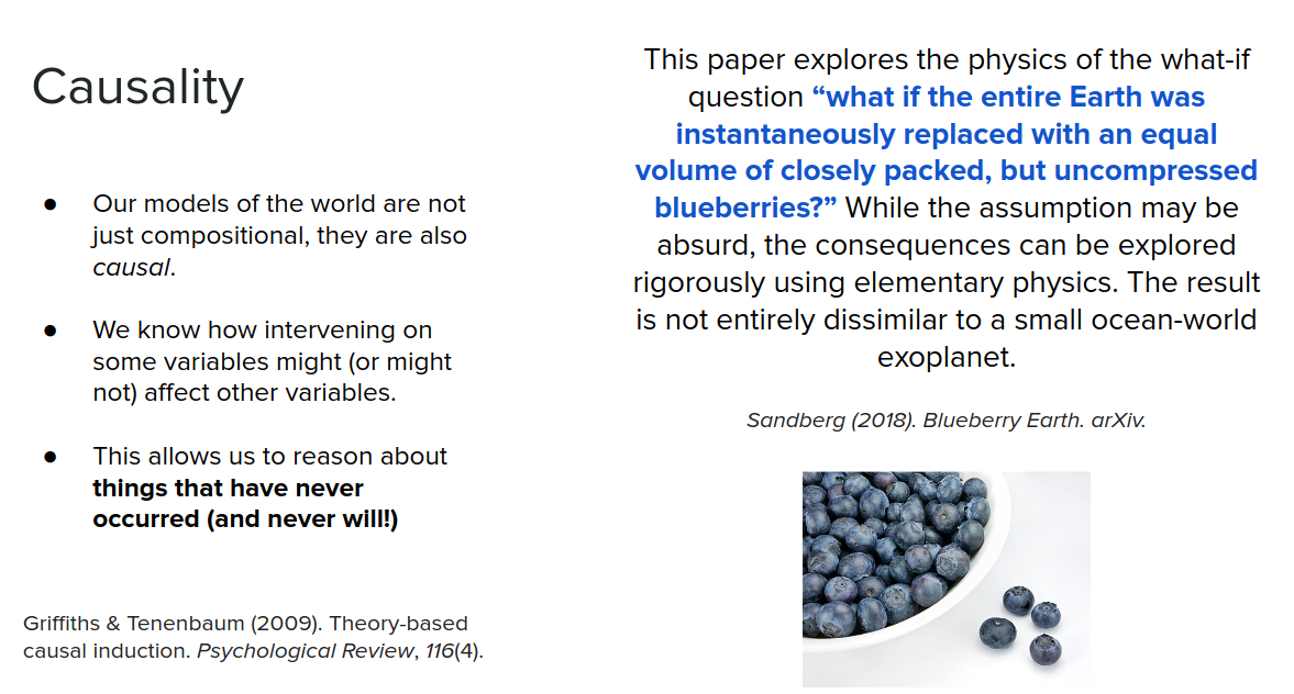
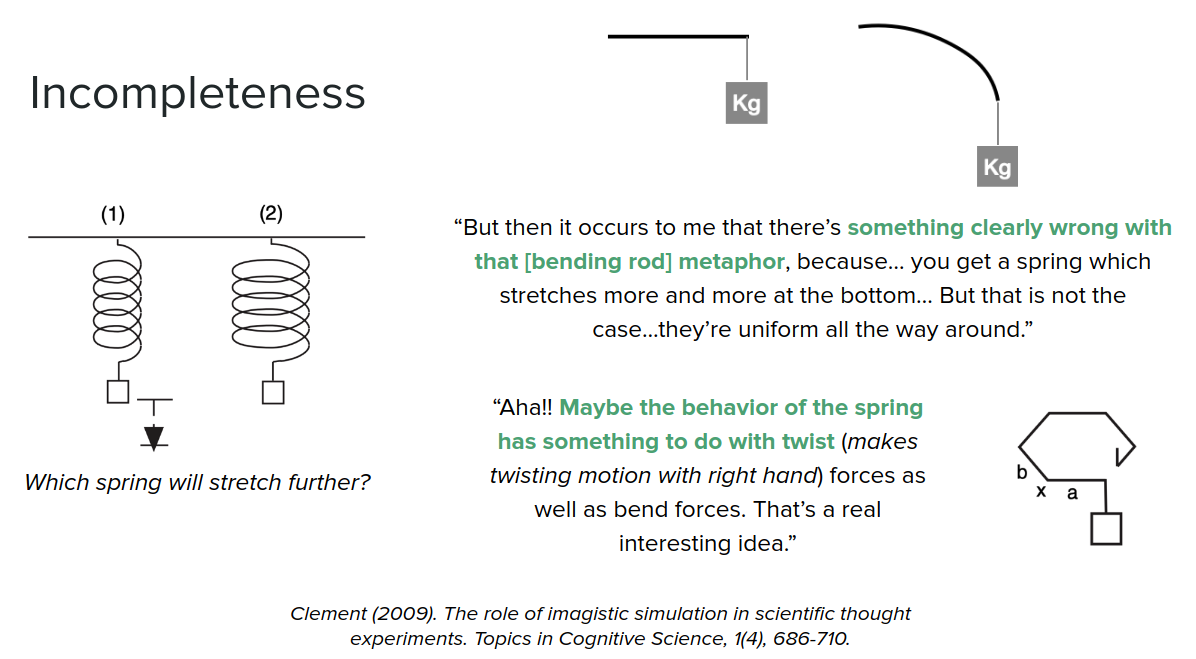
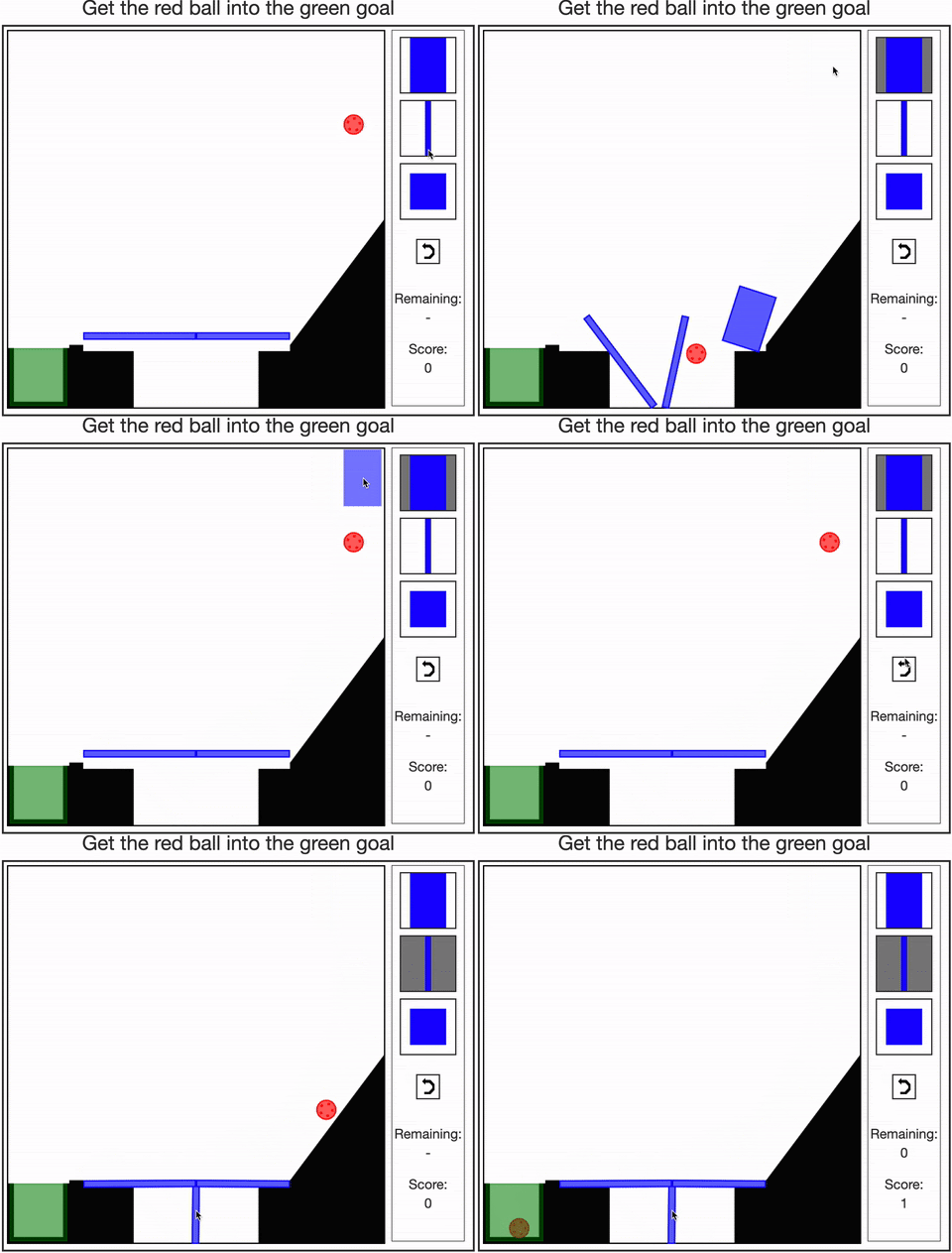
Humans use their models of the world in ways that are compositional, causal, incomplete, adaptive, efficient, and abstract. Taking these ideas and trying to distill them into MBRL enables us to do

faster planning
have systems with higher tolerance to model error
can be scaled to much much harder problems.

This will lead us to more robust real-world applications and better common sense reasoning.

Compositionality

Humans are much much stronger than MBRL algorithms that we have in compositionality.

Causality

Incompleteness

Another facet of human model based reasoning in the fact that we can reason about incomplete models, but reason about them in very tich ways. This is in contrast to model-based RL which if we have model error, it would be a huge deal and are very far from human capabilities.

Adaptivity

The way that we (humans) use our models is also incredibly adaptive. We can rapidly assemble our compositional knowledge into on-the-fly models that are adapted to the current task. Then we quickly solve these models, leveraging both mental simulation & (carefully chosen) real experience

Allen, Smith, & Tenenbaum (2019). The tools challenge: Rapid trial-and-error learning in physical problem solving. CogSci 2019.
Dasgupta, Smith, Schulz, Tenenbaum, & Gershman (2018). Learning to act by integrating mental simulations and physical experiments. CogSci 2018.

Efficiency

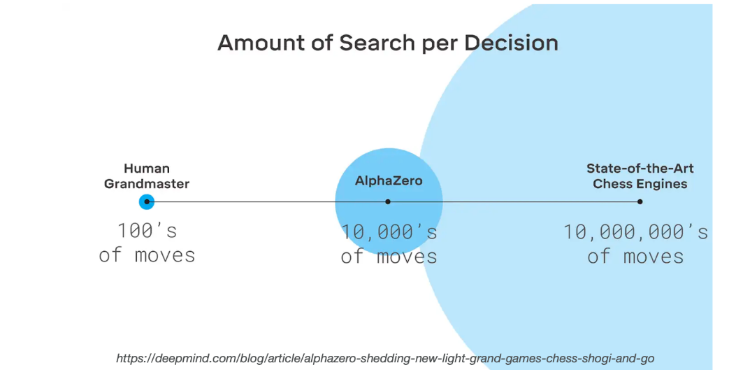
Humans' model-based reasoning is also very efficient. Figure below illustrates how much of an improvement Alpha-zero was over former state of the art chess engine which requires a tens of millions of moves during simulation. Whereas Alpha-zero only needs tens of thousands. But again it is not comparable to human grandmaster, which only requires hundreds of moves. So we need to continue to develop planners that are able to sort of leverage our models as quickly and as efficiently as possible towards this type of efficiency.

Abstraction

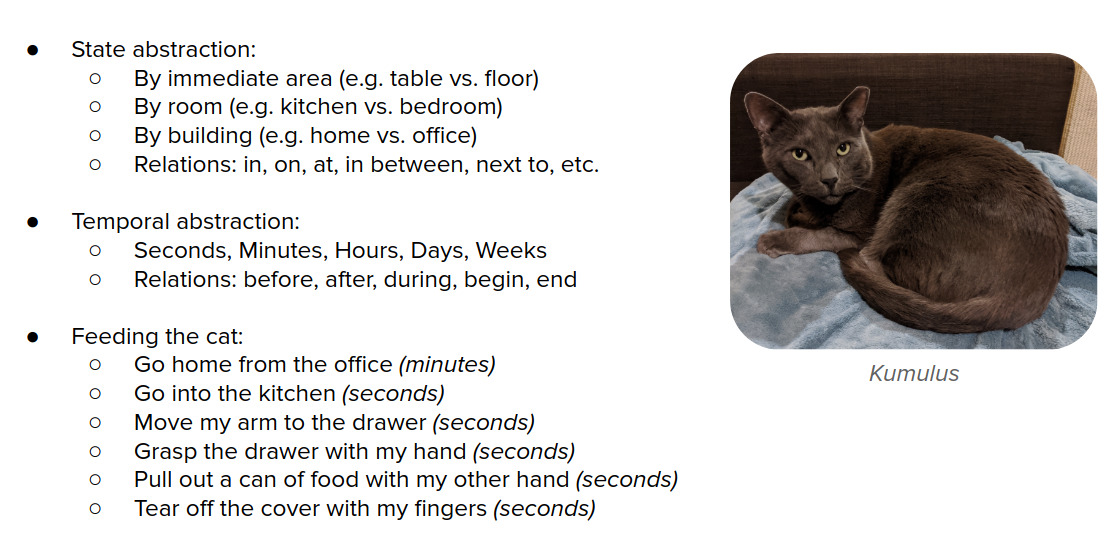
The final feature of humans' ability to use models of the world is abstraction. We go through all of different levels of abstraction as we're planning over multiple timescales, over multiple forms of state abstraction, and we move up and down different forms of abstraction as needed and so we ideally want integrated agents that could do the same.

Conclusion

In this tutorial, we discussed what it means to have a model of the world and different types of models that you can learn. We also talked about where the model fits into the RL loop. We talked about landscape of model-based methods and some practical considerations that we care about when integrating models into the loop. We also saw how we can try to improve models by looking towards human cognition.

Ethical and broader impacts

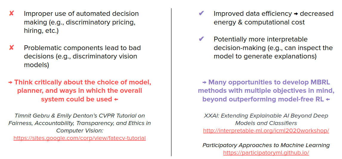
Because MBRL inherits methods both from model-free RL and model learning in general, it inherits the problems from both of them too.