MLOps project - part 4a: Machine Learning Model Monitoring
Monitoring deployed machine learning models in production.


Note: The majority of the information in this blog post comes from the documentations and talks of the tools' authors and creators. I simply put them together. The details of each company's solutions depend on the information contained in their documentation and online discussions.
After several years of research and development in laboratories, machine learning models are increasingly entering production. The topic of deploying the designed machine learning models into production will be covered in a subsequent post. However, a machine learning model's existence does not end upon deployment. Monitoring the model and ensuring that it fulfills its responsibilities emerges after deployment.
In this article, we will discuss different monitoring solutions for machine learning models in production. We will analyze how various solutions can assist us in determining whether the model performs as expected and, if not, what should be done. Let's get started!
First, let's see what is machine learning model monitoring?
Machine learning model monitoring is a practice of tracking and analyzing production model performance to ensure acceptable quality as defined by the use case. It provides early warnings on performance issues and helps diagnose their root cause to debug and resolve. [source] Many things can go wrong with data and model in a machine learning service that are not detectable by old and conventional software monitoring tools. Issues such as data pipeline, data quality, inference service latency, model accuracy, and many more. Checking business metrics and KPIs may be too late to figure out the machine learning service problems. In addition, failure to discover these issues proactively can have a major negative impact on corporate performance and credibility to the end-user. Therefore, detecting these kinds of problems and acting on time would be very important.
I can't recommend a website more than the EvidentlyAI blog posts to learn about machine learning model monitoring concept. I also found This blog post by Aporia and this one by Seldon useful.
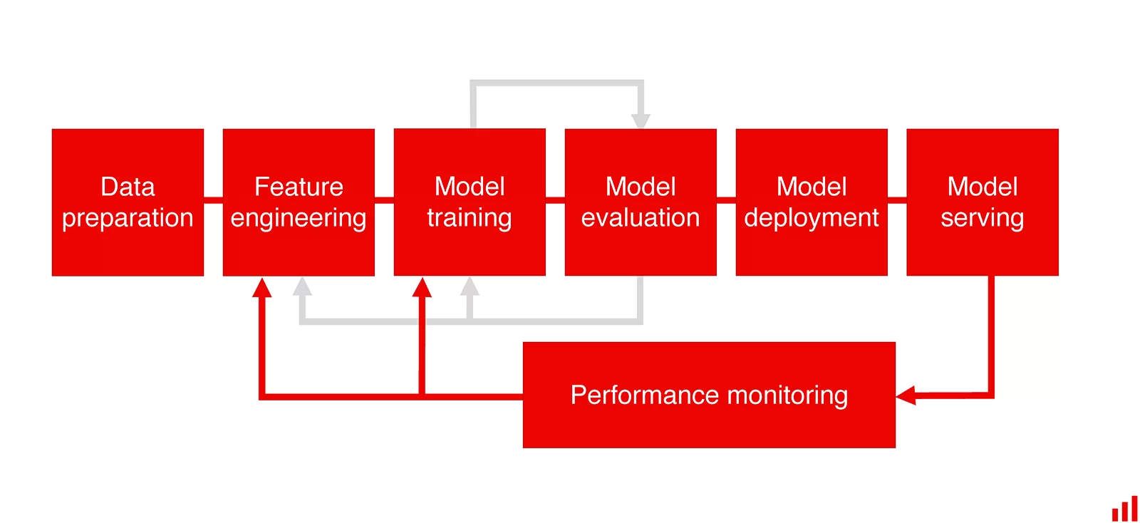
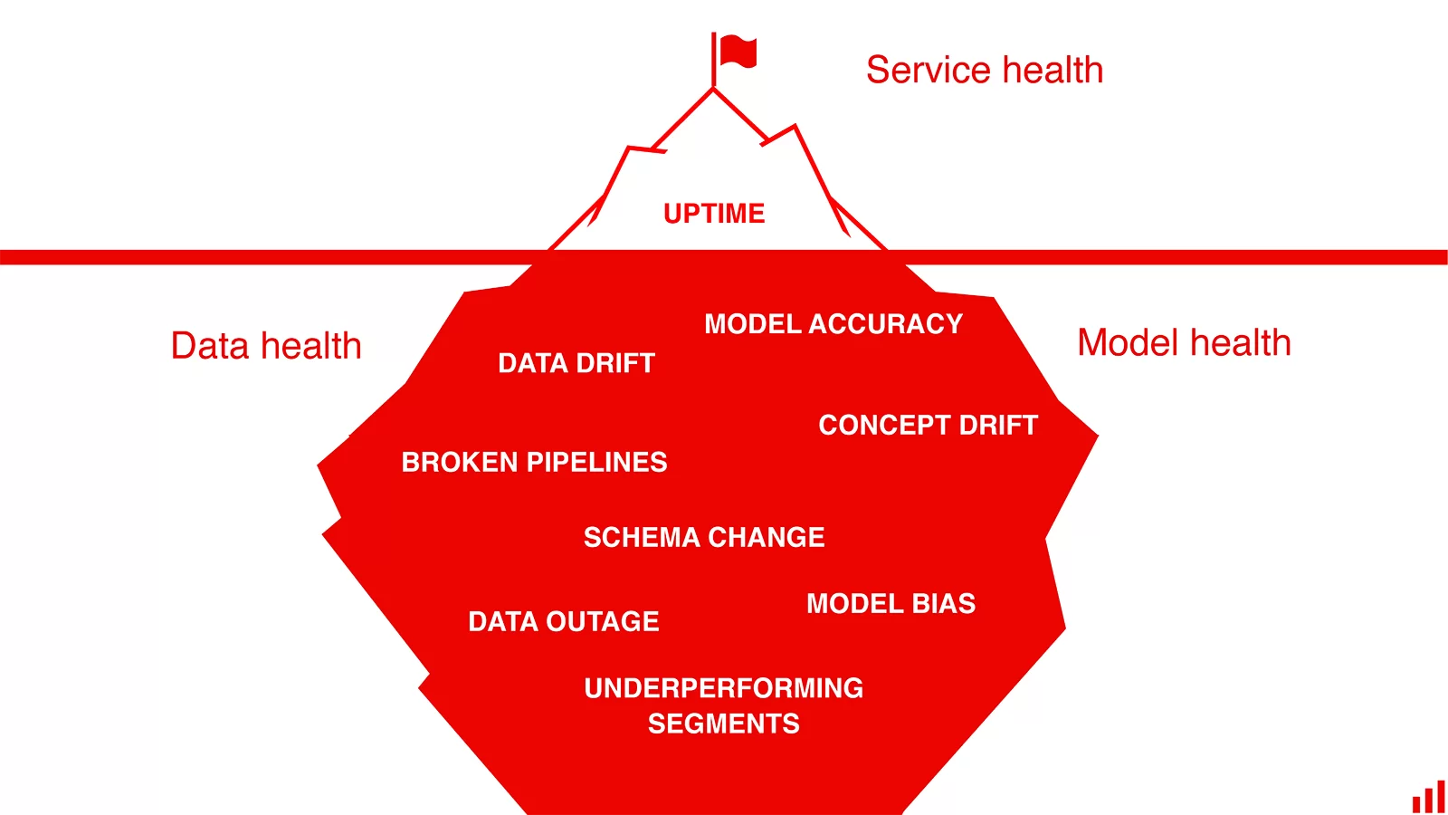
All models degrade. There are different categories of the problems that can happen to a machine learning service.
- Sometimes, poor data quality, broken pipelines, or technical bugs cause a performance drop.
- Sometimes data drift, which is the change in data distributions -> The model performs worse on unknown data regions.
- And sometimes it is concept drift, which is the change in relationships -> The world has changed, and the model needs an update. It can be gradual (expected), sudden (you get it), and recurring (seasonal).
For more details, read the references I mentioned above or at the end of the blog post. Let's go for solutions and tools for ML model monitoring.
Evidently AI
Evidentlyai is one of the hottest startups working in this topic. Based on their documentations, Evidently generates interactive dashboards from pandas DataFrame or csv files, which can be used for model evaluation, debugging and documentation.
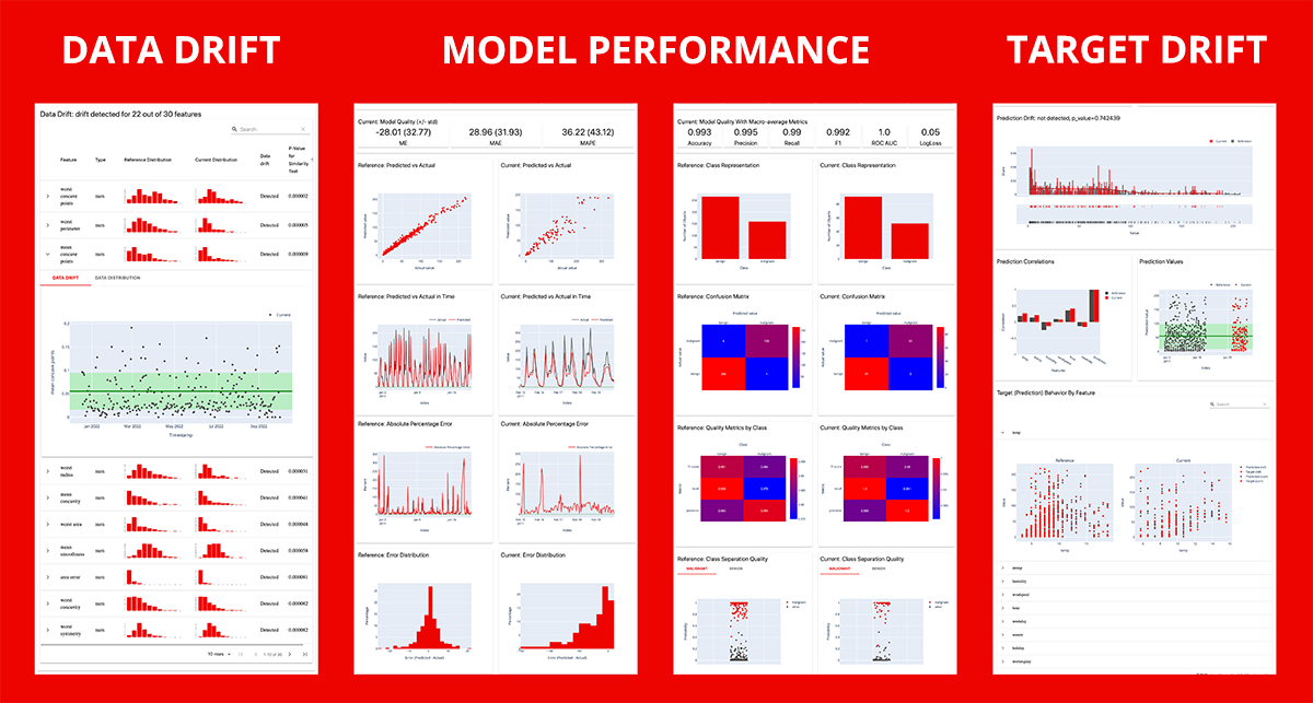
Each report covers a particular aspect of the model performance. Currently 7 pre-built reports are available:
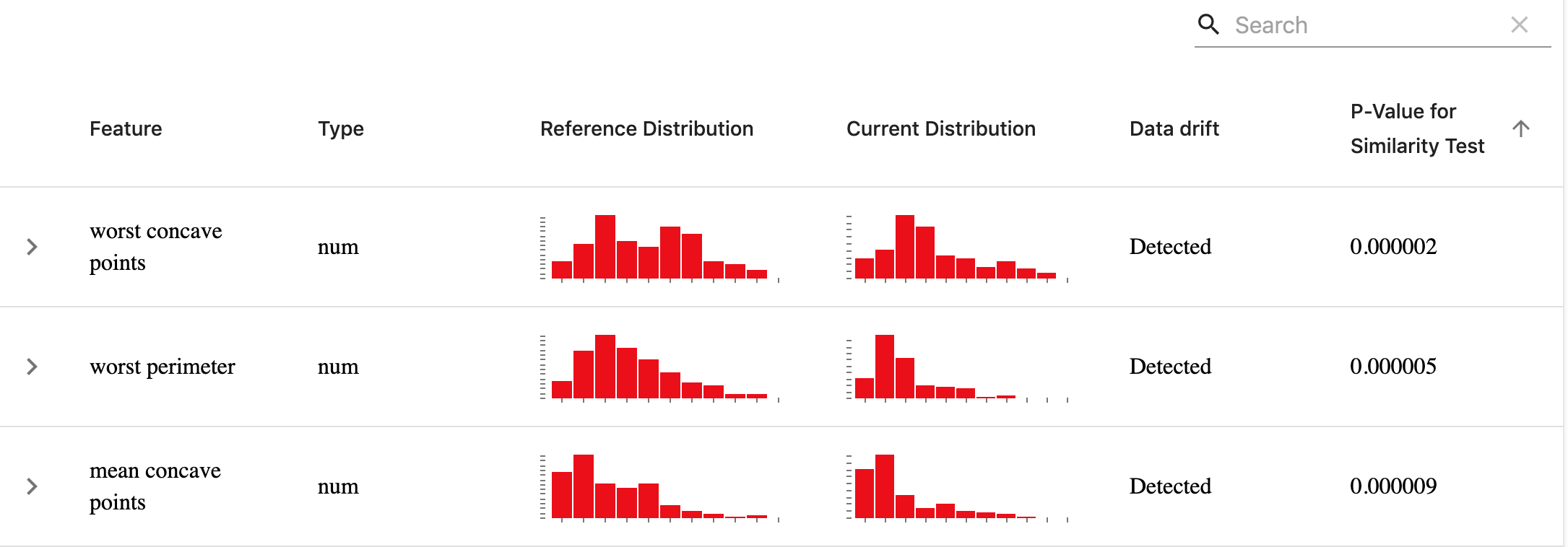
- Data Drift: Detects changes in the input feature distribution. You'll require two datasets. The benchmark dataset is the reference set. By comparing the current production data to the reference data, they analyze the change. To estimate the data drift Evidently c ompares the distributions of each characteristic in the two datasets. Evidently employs statistical tests to determine if the distribution has significantly shifted.
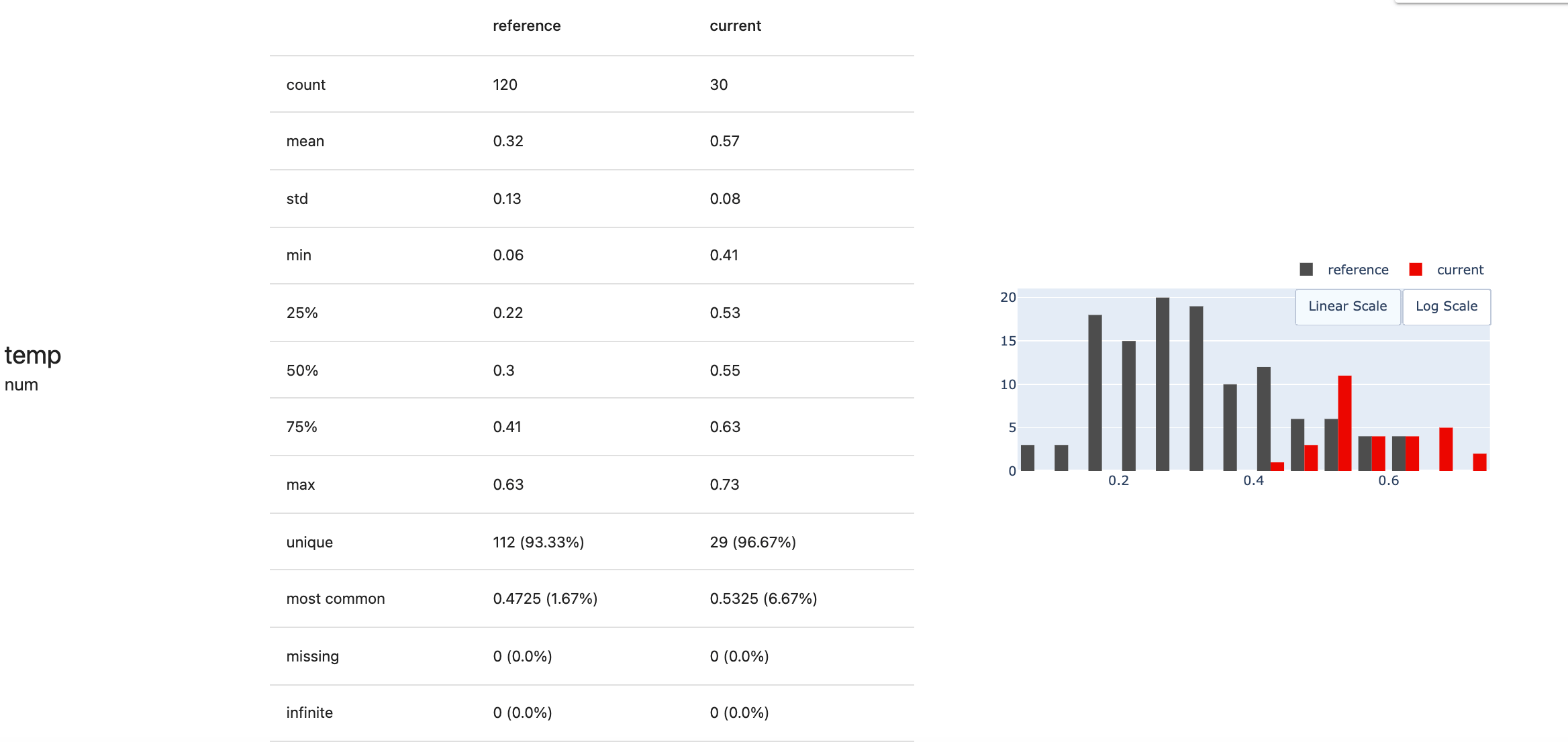
- Data Quality: Provides detailed feature statistics and behavior overview. Additionally, it can compare any two datasets. It can be utilized to compare train and test data, reference and current data, or two subsets of a single dataset (e.g., customers in different regions).
- Target Drift:
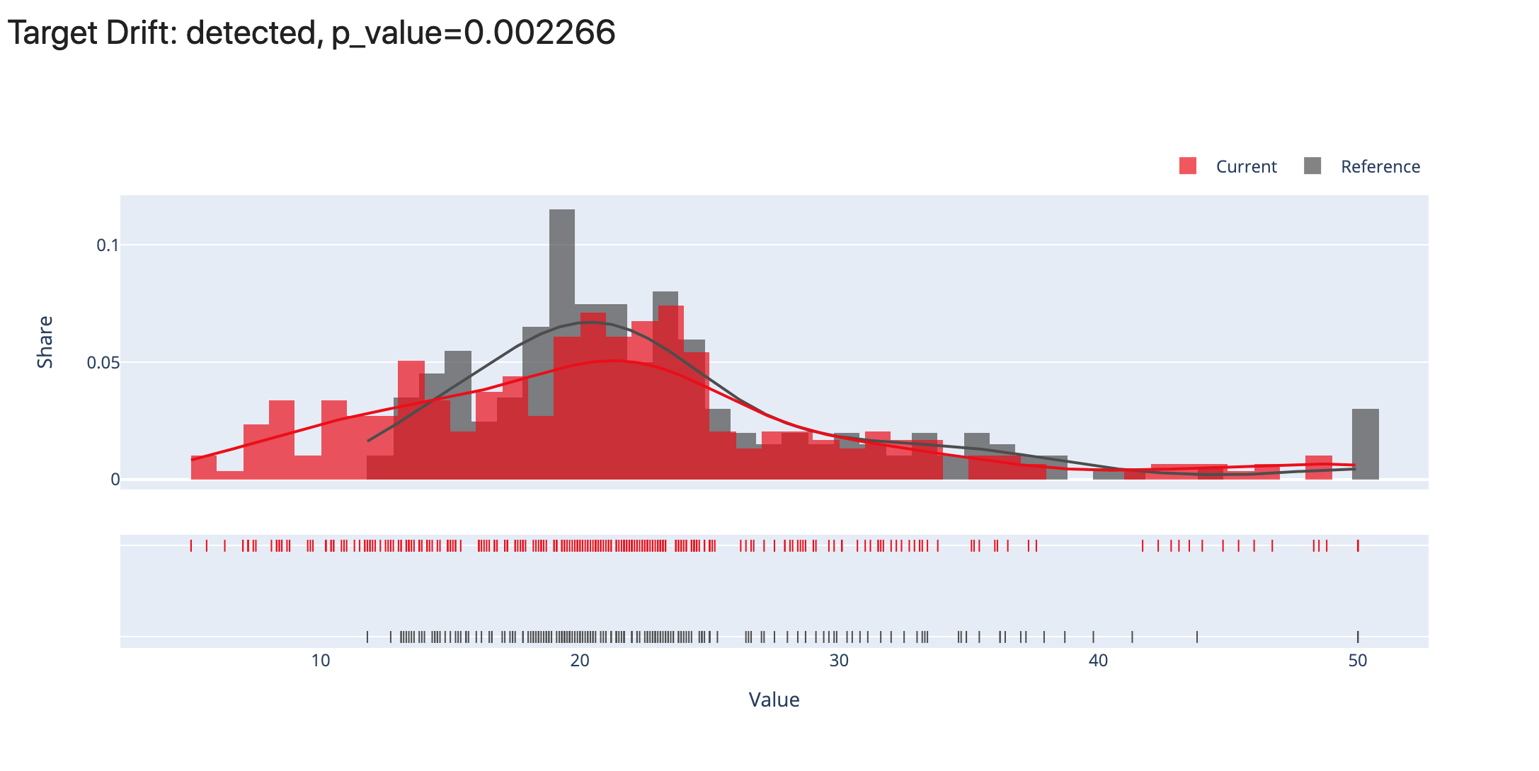
Numerical: The Target Drift report assists in identifying and investigating changes to the target function and/or model predictions. The Numerical Target Drift report is appropriate for problem statements with a numerical target function, such as regression, probabilistic classification, and ranking, among others. To run this report, you must have available input features, target columns, and/or prediction columns. You'll require two datasets. The benchmark dataset is the reference set. By comparing the current production data to the reference data, they analyze the change.
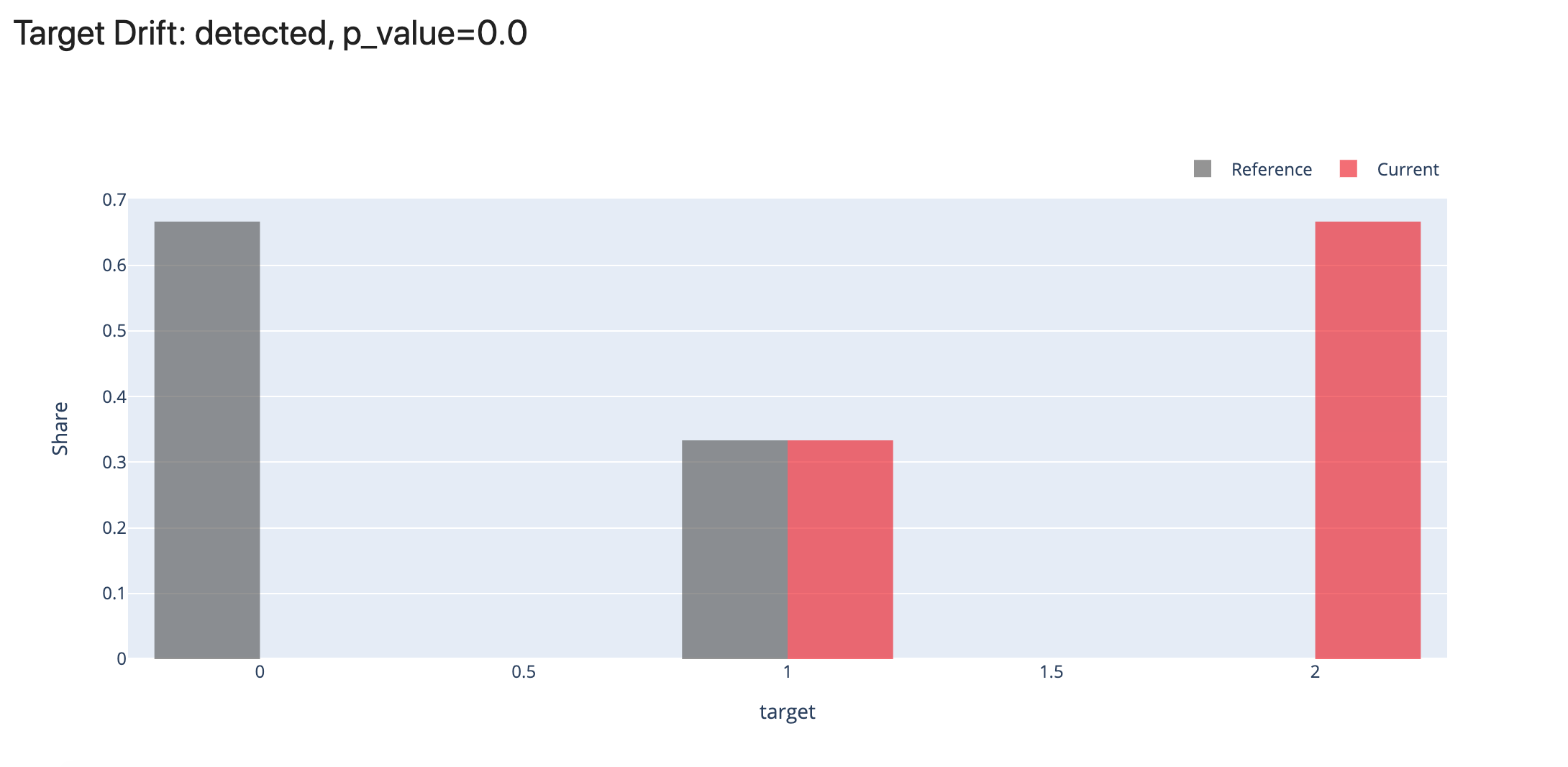
Categorical: Categorical Target Drift is appropriate for problem statements with a categorical target function, such as binary classification, multi-class classification, etc. To run this report, you must have available input features, target columns, and/or prediction columns. You'll require two datasets. The benchmark dataset is the reference set. By comparing the current production data to the reference data, they analyze the change.
- Model Performance:
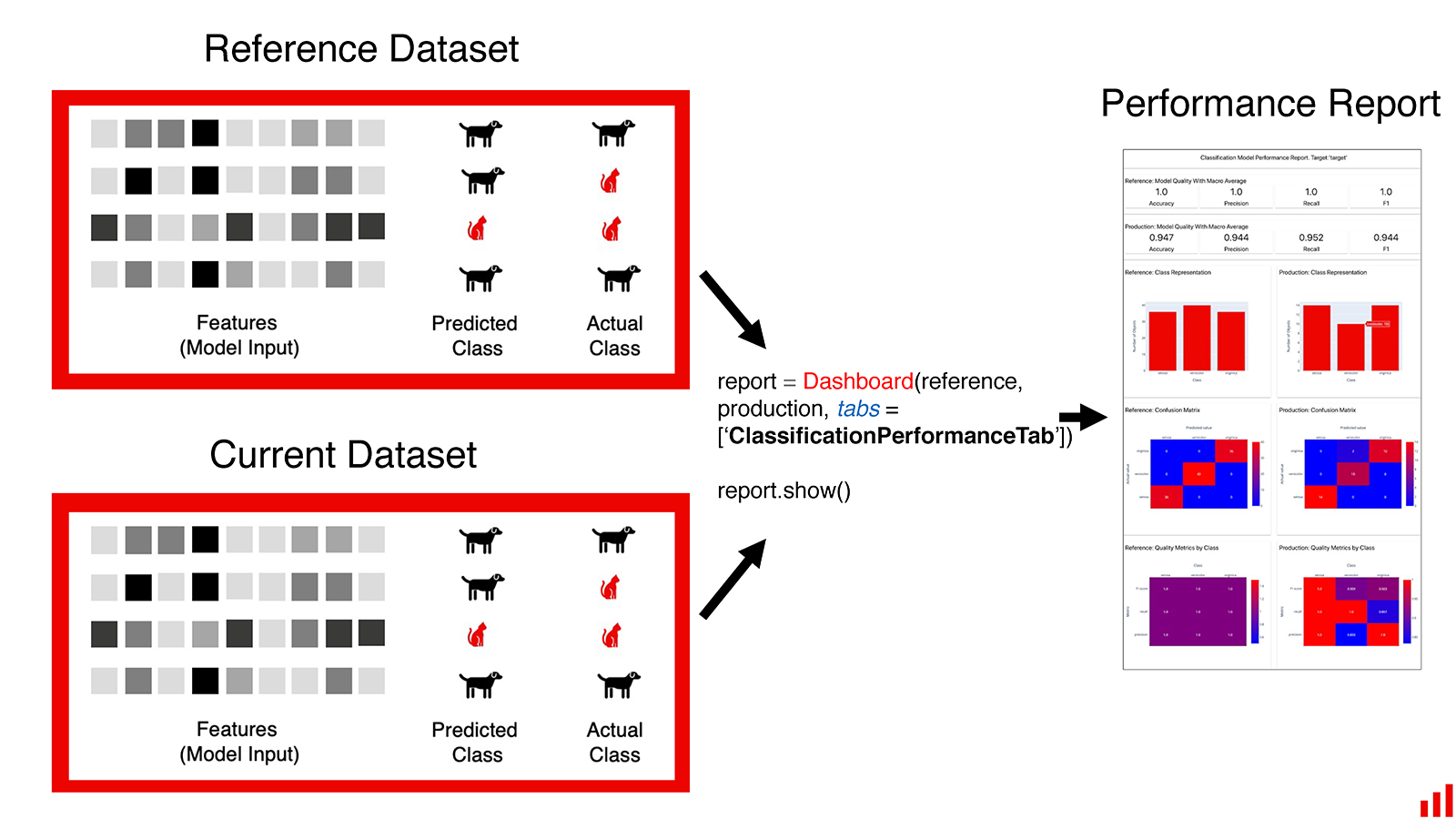
Classification: Classification Performance report evaluates a classification model's quality. It is applicable for both binary and multiclass classification. This report can be generated for a single model or as a comparison between two models. You can compare the performance of your current production model to that of a previous model or an alternative model. To run this report, you must have available input features, target columns, and prediction columns.

Probabilistic Classification: The Probabilistic Classification Performance report evaluates a probabilistic classification model's quality. It is applicable for both binary and multiclass classification. This report can be generated for a single model or as a comparison between two models. You can compare the performance of your current production model to that of a previous model or an alternative model. To run this report, you must have available input features, target columns, and prediction columns.
Regression: The Regression Performance report evaluates a regression model's quality. It can also compare it to the performance of the same model in the past or to the performance of a different model. To run this report, you must have available input features, target columns, and prediction columns. To generate a comparative report, two datasets are required. The benchmark dataset is the reference set. By comparing the current production data to the reference data, they analyze the change.
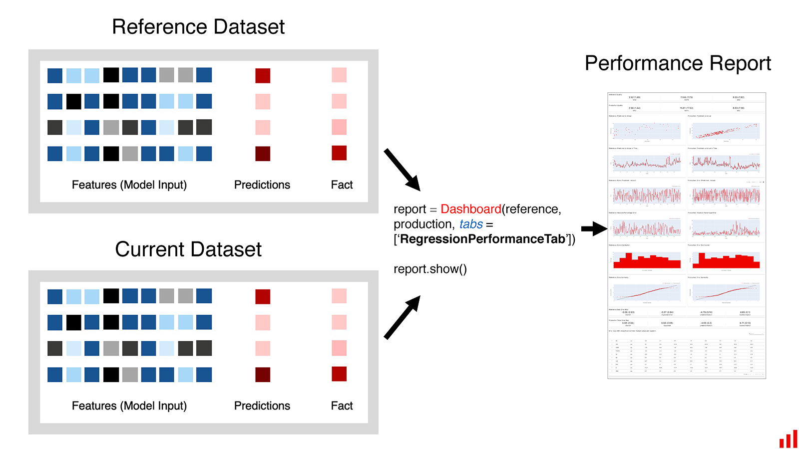
Again, I highly recommend reading their blog posts for more details. We just reviewed a small portion here. Now let's see a small demo of data drift and numerical target drift on California Housing dataset:
import pandas as pd

from sklearn.datasets import fetch_california_housing

from evidently.dashboard import Dashboard
from evidently.pipeline.column_mapping import ColumnMapping
from evidently.dashboard.tabs import DataDriftTab, NumTargetDriftTab

from evidently.model_profile import Profile
from evidently.model_profile.sections import DataDriftProfileSection, NumTargetDriftProfileSection

%matplotlib inline
import warnings
warnings.filterwarnings('ignore')
warnings.simplefilter('ignore')
ca = fetch_california_housing(as_frame=True)
ca_frame = ca.frame
ca_frame.head()
target = 'MedHouseVal'
numerical_features = ['MedInc', 'HouseAge', 'AveRooms', 'AveBedrms', 'Population', 'AveOccup',
                      'Latitude', 'Longitude']
categorical_features = []
features = numerical_features

column_mapping = ColumnMapping()
column_mapping.target = target
column_mapping.numerical_features = numerical_features

ref_data_sample = ca_frame[:15000].sample(1000, random_state=0)
prod_data_sample = ca_frame[15000:].sample(1000, random_state=0)

ca_data_and_target_drift_dashboard = Dashboard(tabs=[DataDriftTab(verbose_level=0),
                                                     NumTargetDriftTab(verbose_level=0)])
ca_data_and_target_drift_dashboard.calculate(ref_data_sample, prod_data_sample, column_mapping=column_mapping)
ca_data_and_target_drift_dashboard.show(mode='inline')
The negative point about EvidentlyAI is that it doesn't support data types like image and text.
Seldon ALIBI Detect
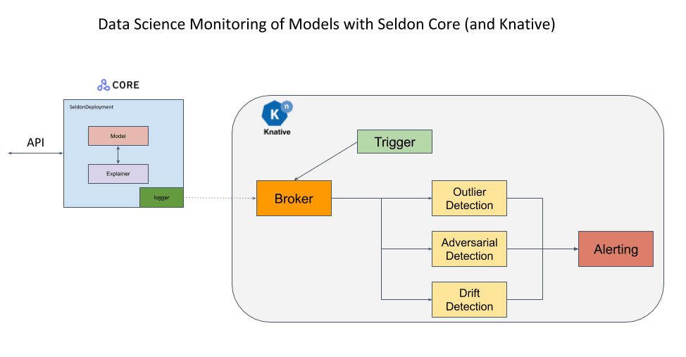
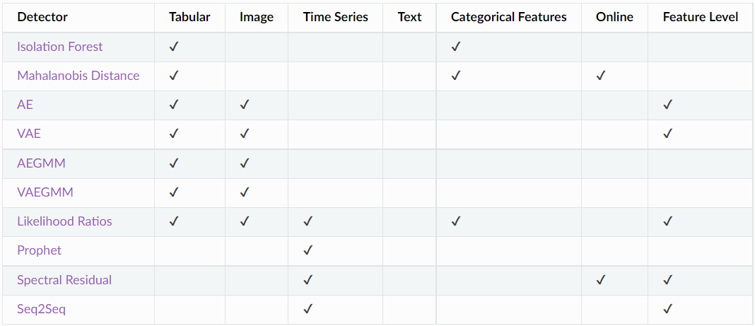
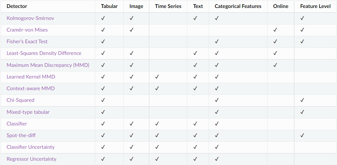
Seldon is another amazing tool. They have many services and one of them is called ALIBI DETECT. Alibi Detect is a Python library that focuses on outlier, adversarial, and drift detection. The goal of the package is to include both online and offline detectors for tabular data, text, images, and time series. For drift detection, both TensorFlow and PyTorch backends are supported. They have laso implemented state-of-the-art techniques for each one of outlier, drift, and adversarial attack detection. The following summary tables shows the practical use cases for all the algorithms.
Outlier detection
I just explain some of them here:
-
Auto-Encoder: The Auto-Encoder (AE) outlier detector is initially trained using unlabeled but normal (inlier) data. Rarely available labeled data makes unsupervised training desirable. The AE detector attempts to reconstruct the received input. If the input data cannot be accurately reconstructed, the reconstruction error is high and the data can be flagged as an outlier. Mean squared error (MSE) is used to measure the reconstruction error between the input and the reconstructed instance.
-
Auto-Encoding Gaussian Mixture Model: The encoder compresses the data, while the reconstructed instances generated by the decoder are used to create additional features based on the reconstruction error between the input and reconstructions. These features are combined with encodings and fed into a Gaussian Mixture Model (GMM). The AEGMM outlier detector is initially trained using unlabeled but normal (inlier) data. Rarely available labeled data makes unsupervised or semi-supervised training desirable. The sample energy of the GMM can then be used to determine whether a given instance is an outlier (high sample energy) or not (low sample energy). The algorithm is compatible with both tabular and image data types.
-
Prophet Detector: The Prophet outlier detector employs the Prophet time series forecasting package. Combining trend, seasonality, and holiday effects, the underlying Prophet model is a decomposable univariate time series model. The model forecast also includes an uncertainty interval around the estimated trend component derived from the extrapolated model's MAP estimate. Alternately, complete Bayesian inference can be performed at the expense of a greater computational cost. The maximum and minimum values of the uncertainty interval can then be utilized as outlier thresholds for each time point. First, the distance between the observed value and the nearest uncertainty boundary (upper or lower) is computed. If the observation falls within the limits, the outlier score equals the negative distance. Therefore, the outlier score is lowest when the observation and model prediction coincide. If the observation is outside the boundaries, the score is equal to the distance measure, and the observation is marked as an outlier. However, one of the major drawbacks of the method is that the model must be re-fitted whenever new data becomes available. This is undesirable for applications with real-time detection and high throughput.
-
Spectral Residual: This method is appropriate for unsupervised online detection of anomalies in univariate time series data. First, the algorithm calculates the Fourier Transform of the initial data. Before applying the Inverse Fourier Transform to map the sequence back from the frequency domain to the time domain, the spectral residual of the transformed signal's log amplitude is computed. This sequence is referred to as the saliency map. The anomaly score is then calculated as the relative difference of the the saliency map values to their moving averages. If the score is greater than a predetermined threshold, the value at a particular timestep is marked as an outlier.
For more details and also to become more familiar with other algorithms for outlier detection, please check their documentation and reference papers.
Adversarial Detection
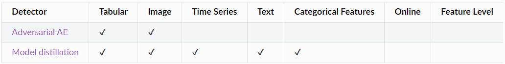
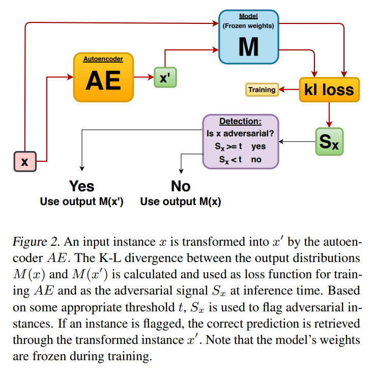
- Adversarial Auto-Encoder: The detector is an autoencoder trained with a custom loss function based on the Kullback-Leibler divergence between classifier predictions on original and reconstructed instances. The method is unsupervised, simple to train, and does not require knowledge of the attack's underlying mechanism. The detector almost completely neutralizes powerful attacks such as Carlini-Wagner or SLIDE on MNIST and Fashion-NIST, and it remains highly effective on CIFAR-10 even when the attacker has full access to the classification model but the defense does not.
- Model distillation: Model distillation is a technique that is used to transfer knowledge from a large network to a smaller network. Typically, it consists of training a second model with a simplified architecture on soft targets (the output distributions or the logits) obtained from the original model. Here, we apply model distillation to obtain harmfulness scores, by comparing the output distributions of the original model with the output distributions of the distilled model, in order to detect adversarial data, malicious data drift or data corruption.
Drift Detection
-
Fisher’s Exact Test: The FET drift detector is a non-parametric drift detector. It applies Fisher’s Exact Test (FET) to each feature, and is intended for application to Bernoulli distributions, with binary univariate data consisting of either (True, False) or (0, 1). This detector is ideal for use in a supervised setting, monitoring drift in a model’s instance level accuracy (i.e. correct prediction = 0, and incorrect prediction = 1).
-
The Maximum Mean Discrepancy: The Maximum Mean Discrepancy (MMD) detector is a kernel-based method for multivariate 2 sample testing. The MMD is a distance-based measure between 2 distributions p and q based on the mean embeddings in a reproducing kernel Hilbert space
-
Learned Kernel: The learned-kernel drift detector is an extension of the Maximum Mean Discrepancy drift detector where the kernel used to define the MMD is trained using a portion of the data to maximise an estimate of the resulting test power. Once the kernel has been learned a permutation test is performed in the usual way on the value of the MMD.
-
Chi-Squared: The drift detector applies feature-wise Chi-Squared tests for the categorical features. For multivariate data, the p-values for each characteristic are aggregated using either the Bonferroni or False Discovery Rate (FDR) correction. The Bonferroni correction is more conservative and controls for at least one false positive probability. In contrast, the FDR correction permits an expected proportion of false positives to occur.
For more details and also other methods, please refer to their documentations and reference papers. I also recommend reading their amazing documentation about drift here. They have also a lot of examples on image, text, graph, etc. problems.
Let's see an example of Categorical and mixed type data drift detection on income prediction. The instances contain a person’s characteristics like age, marital status or education while the label represents whether the person makes more or less than $50k per year. The dataset consists of a mixture of numerical and categorical features.
import alibi
import matplotlib.pyplot as plt
import numpy as np

from alibi_detect.cd import ChiSquareDrift, TabularDrift
from alibi_detect.saving import save_detector, load_detector

adult = alibi.datasets.fetch_adult()
X, y = adult.data, adult.target
feature_names = adult.feature_names
category_map = adult.category_map

n_ref = 10000
n_test = 10000

X_ref, X_t0, X_t1 = X[:n_ref], X[n_ref:n_ref + n_test], X[n_ref + n_test:n_ref + 2 * n_test]

categories_per_feature = {f: None for f in list(category_map.keys())}

cd = TabularDrift(X_ref, p_val=.05, categories_per_feature=categories_per_feature)

preds = cd.predict(X_t0)
labels = ['No!', 'Yes!']
print('Drift? {}'.format(labels[preds['data']['is_drift']]))
Let’s take a closer look at each of the features. The preds dictionary also returns the K-S or Chi-Squared test statistics and p-value for each feature:
for f in range(cd.n_features):
    stat = 'Chi2' if f in list(categories_per_feature.keys()) else 'K-S'
    fname = feature_names[f]
    stat_val, p_val = preds['data']['distance'][f], preds['data']['p_val'][f]
    print(f'{fname} -- {stat} {stat_val:.3f} -- p-value {p_val:.3f}')
None of the feature-level p-values are below the threshold:
preds['data']['threshold']
If you are interested in individual feature-wise drift, this is also possible:
fpreds = cd.predict(X_t0, drift_type='feature')
for f in range(cd.n_features):
    stat = 'Chi2' if f in list(categories_per_feature.keys()) else 'K-S'
    fname = feature_names[f]
    is_drift = fpreds['data']['is_drift'][f]
    stat_val, p_val = fpreds['data']['distance'][f], fpreds['data']['p_val'][f]
    print(f'{fname} -- Drift? {labels[is_drift]} -- {stat} {stat_val:.3f} -- p-value {p_val:.3f}')
Other references:
https://censius.ai/wiki

https://censius.ai/mlops
https://docs.aporia.com/
https://www.aporia.com/machine-learning-model-monitoring-101/
https://github.com/whylabs/whylogs
Amazon SageMaker Model Monitoring
Amazon SageMaker is a fully managed service that removes the manual labor from each step of the machine learning process by utilizing decoupled modules for collecting and preparing data, training and tuning a model, deploying the trained model, and monitoring the models deployed in production.
SageMaker's deploying module enables the hosting of real-time inference endpoints. We will focus on monitoring the endpoints of the production model.
Machine learning models are typically trained and evaluated using historical data. However, the real-world data may not resemble the training data, particularly as models age and data distributions change. For instance, the inputted data units may change from Fahrenheit to Celsius, or your application may start sending null values to your model, which has a significant impact on model quality. Or perhaps, in a real-world retail scenario, consumers' purchasing preferences evolve over time. This gradual misalignment between the model and the real world is known as model drift or data drift, and it can have a significant effect on the accuracy of predictions. Similarly, the performance of the model may decline over time. Degradation of model accuracy with time has an effect on business outcomes. Continuous monitoring of the model's performance is vital for proactively addressing this issue.
This continuous monitoring enables you to determine the optimal time and frequency for retraining your machine learning model. While frequent retraining can be prohibitively expensive, infrequent training may result in less-than-optimal predictions from your machine learning model. So acting on the right time is valuable here.
Model monitoring emits metrics into Amazon Cloud Watch when some defined rules and thresholds are violated, allowing you to set up alarms to audit and retrain models. Metrics for data drift and accuracy drift are also stored in S3 buckets and can be visualized using SageMaker Studio.
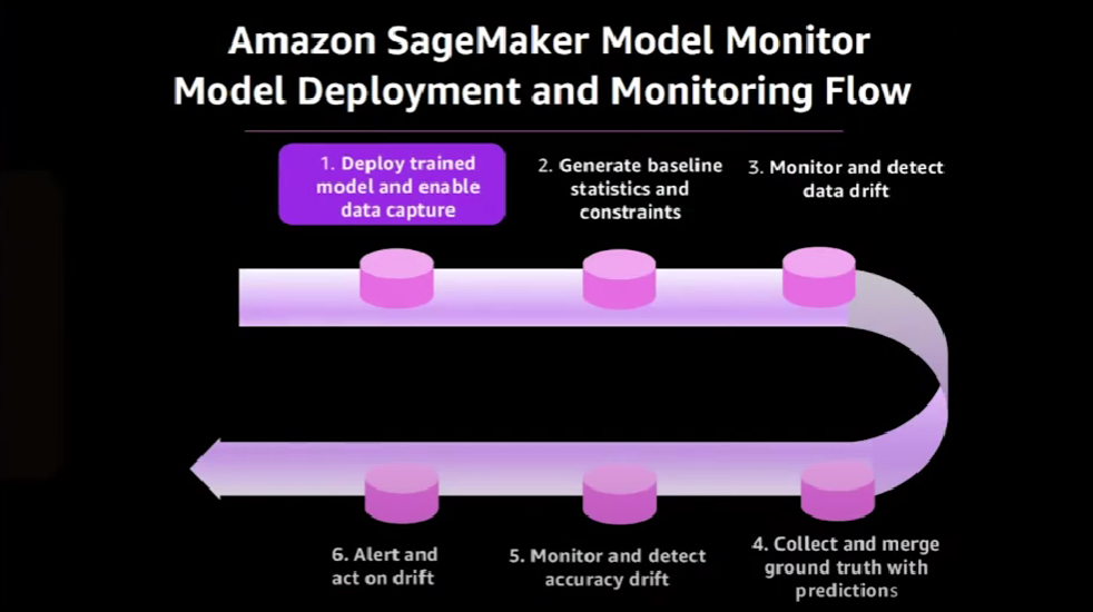
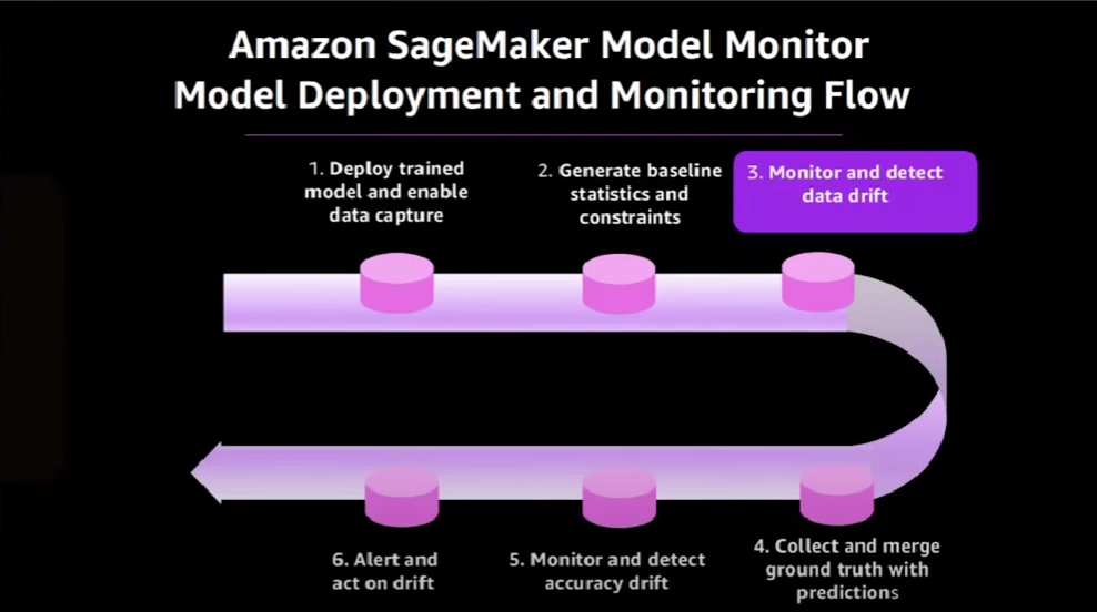
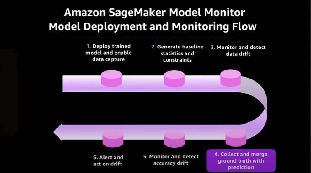
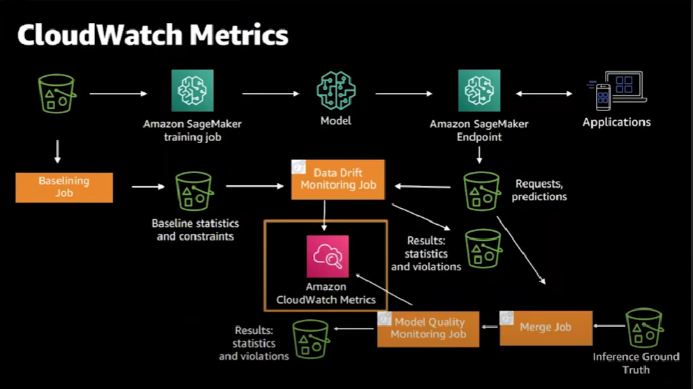
An end-to-end flow for deploying and monitoring models in production in Amazon SageMaker looks like this:
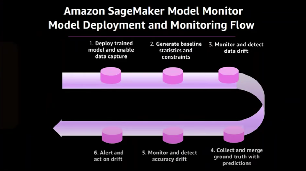
It begins with deploying the trained model and concludes with corrective action being taken once drift has been detected. Here is the end-to-end architecture that corresponds to that end-to-end flow.
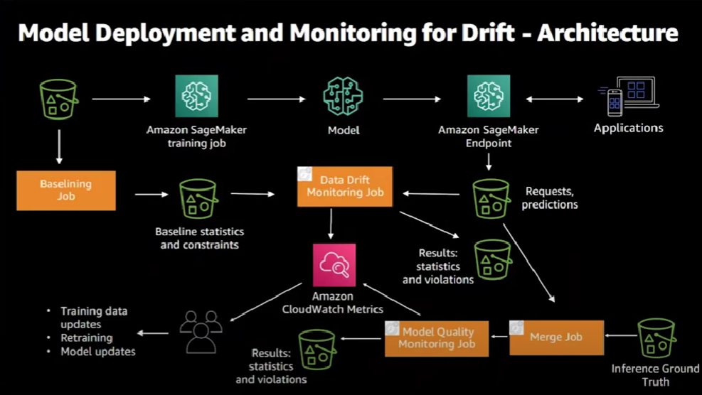
Let's analyze this diagram in more details. The first step is to deploy the trained model.
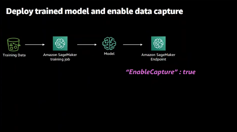
We start with ground truth training data and run a training job on SageMaker, which generates a model artifact. Then the trained model would be available to consumers via a deployed SageMaker endpoint.
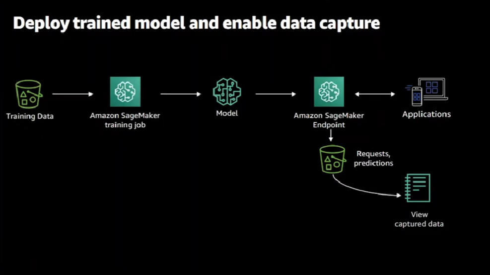
Now, with the endpoint deployed, a consuming application can start sending requests and get back predictions from the model. Then the request and the responses are captured in S3.
In order to identify if there's any kind of data drift, we need to have some baseline data.
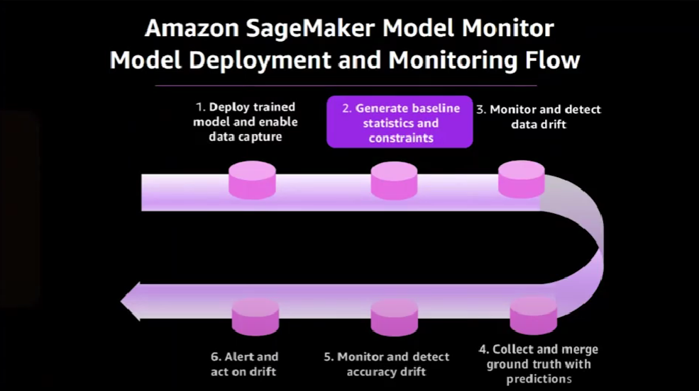
In the next step, we run a baselining job that generates the statistics and constraints about the training data.
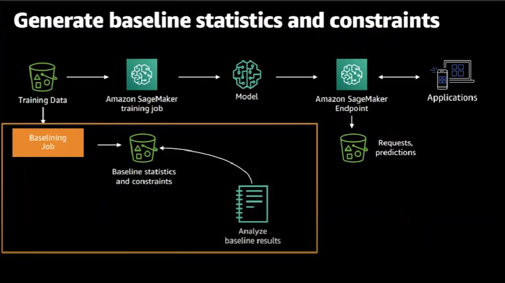
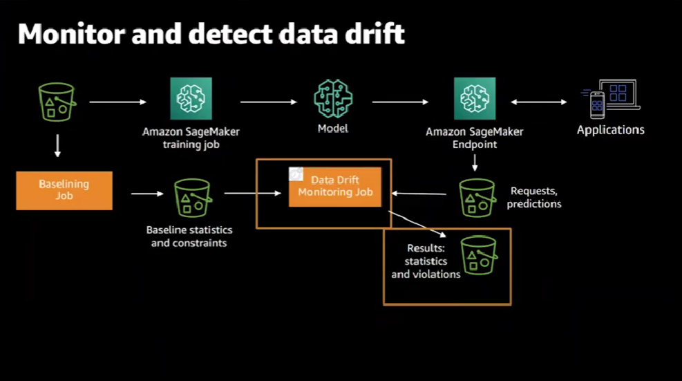
Then we can create a data drift monitoring job that SageMaker will periodically run at a schedule that we can set.
The job compares the inference requests to the statistics and constraints of the baseline. For each execution of the monitoring job, the generated results consist of a violation report that is persisted in Amazon S3, a statistics report of the data collected during the run, and summary metrics and statistics that are sent to Amazon Cloud Watch.
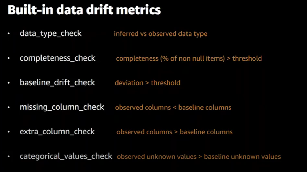
Here are the few violations that are generated.
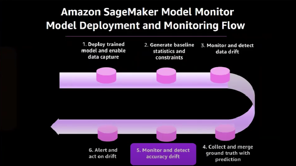
Now we're able to detect data quality drift. But what happens if the quality of the model itself changes? For example, the accuracy of the model decreases. Let's see how to use the Model Monitor capability to detect the accuracy drift.
The process for detecting accuracy drift is almost similar to data drift detection process.
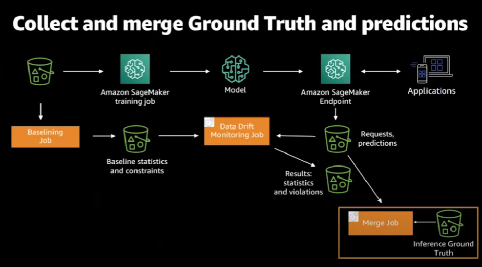
We collect the predictions made and the ground truth of the prediction and compare the two. But what does the inference ground truth mean? What does a prediction ground truth mean? That would depend on the predictions made by your model and the business use case. Consider that you are observing a movie recommendation model. In this case, a possible ground truth inference is whether or not the user has actually watched the recommended film. Or perhaps they simply clicked on the video but did not actually watch it.
With both the predictions captured and ground truth provided by the model consuming application, SageMaker executes a merge job to combine them together. Again, the merge job is a periodic job that is executed according to a schedule.
Once you have the data merged, it's time to monitor the accuracy.
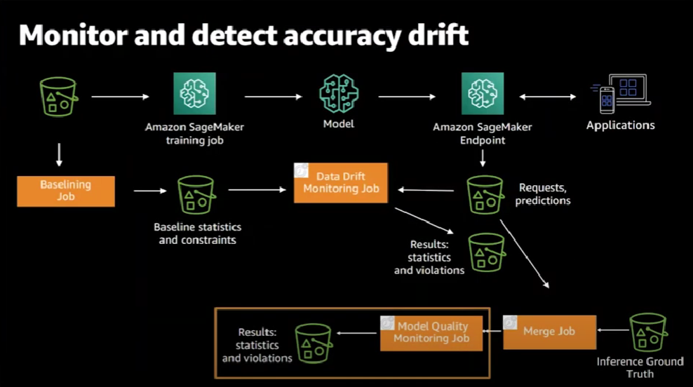
In this step, we can create a model quality monitoring job, which is executed periodically at a schedule. The model quality job generates statistics, violations and Cloud Watch metrics.
The metrics that are generated by the two monitoring jobs can actually be visualized in SageMaker Studio as well.
For the model quality monitoring job, here are some of the metrics that are generated: accuracy, precision, and recall. SageMaker Model Monitor supports classification and regression metrics, but we can also define our own metrics.
After detecting both data and model drifts, it's time to take actions on that.
Both the data drift and the model quality monitoring jobs emit Cloud Watch metrics. We can create Cloud Watch alerts for these metrics based on threshold values and, if those thresholds are violated, Cloud Watch alerts will be raised and we can decide on what actions to take such as updating the model, updating training data, and retraining and updating the model itself.
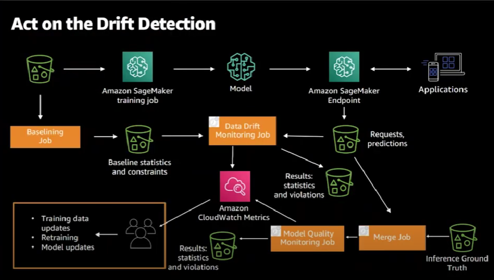
Now, if we decide to retrain the model, we're completing that loop, and can go back to the ground truth training data and start training the model one more time.
Check the following video for more details:
Other resources: