Self-Supervised Monocular Depth Estimation in Autonomous Driving
In this post, I will review self-supervised monocular depth estimation methods.


- Unsupervised Learning of Depth and Ego-Motion from Video
- Digging Into Self-Supervised Monocular Depth Estimation
It is easy for humans to estimate depth in a scene, but what about machines? Typically, robots and self-driving cars use LiDAR sensors to gauge the depth of a scene. However, LiDAR is an expensive sensor that is beyond the reach of many personal vehicles. Robo-Taxis may be reasonable in business models that provide service across a city, but not for personal vehicles. As a result, some companies are using camera-only approaches to infer depth information from monocular images. I will discuss some of the state-of-the-art approaches for monocular depth estimation in this post.
Several approaches are usually used for depth estimation:
-
Geometry-based methods: Geometric constraints are used to recover 3D structures from images. In 3D reconstruction and Simultaneous Localization and Mapping (SLAM) , structure from motion (SfM) is an effective method of estimating 3D structures from a series of 2D image sequences. The accuracy of depth estimation depends heavily on exact feature matching and high-quality image sequences. SfM suffers from monocular scale ambiguity as well. Stereo vision matching is also capable of recovering 3D structures of scenes from two viewpoints. It simulates the way human eyes work by using two cameras, and a cost function is used to calculate disparity maps of images. Due to the calibration of the transformation between the two cameras, the scale factor is incorporated into depth estimation during stereo vision matching.
-
Sensor-based methods: This approach uses sensors such as RGB-D and LiDAR. There are sevaral disadvantages for this method such as cost, power consumption, size of sensor.
-
Deep learning-based methods: The pixel-level depth map can be recovered from a single image in an end-to-end manner based on deep learning. It can be done in supervised, semi-supervised, or self-supervised manner.
In this post, we just consider the self-supervised methods in which the geometric constraints between frames are regarded as the supervisory signal during the training process. There are several types of self-supervised learning methods for estimating depth using images, such as stereo-based and monocular videos. Using methods based on monocular videos presents its own challenges. Along with estimating depth, the model also requires estimating ego-motion between pairs of temporal images during training. The process involves training a pose estimation network, which takes a finite sequence of frames as input and outputs the corresponding camera transformations. Stereo data, however, make the camera-pose estimation a one-time offline calibration but may introduce occlusion and texture-copy artifacts.
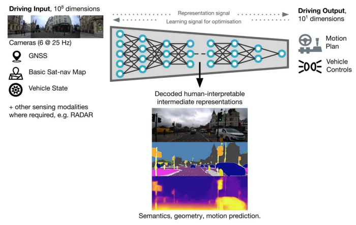
One of the interesting use cases for depth estimation is to use it as an auxiliary task for end-to-end policy learning. It can lead to better representation learning and help the policy to learn some information about the geometric and the depth of the scene. Other tasks, such as optical flow, semantic segmentation, object detection, motion prediction, etc, can also be used to improve representation learning. For example, the following image shows a model from Wayve.ai, a self-driving car company in the UK working on end-to-end autonomous driving, which tries to use multi-task learning to improve representation learning and driving policy learning.
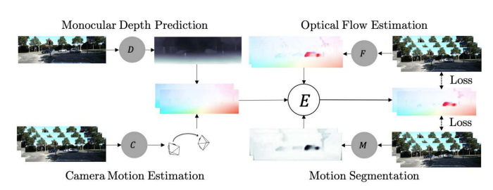
There are also some works that try to learn multiple tasks jointly. Sometimes there is some information in other related tasks that help the networks to learn better. For example, the following work tries to learn optical flow, motion segmentation, camera motion estimation, and depth estimation together:
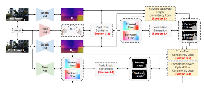
Or the following work that tries to learn optical flow and depth together:
Here in this post, we just want to understand how depth estimation works, and then it would be more straightforward to mix it with other tasks. Maybe in the future, I write other blog posts on other techniques and tasks. In the rest of this post, I will review two related papers for self-supervised monocular depth estimation which use monocular videos and stereo images methods. Let’s get started!
Unsupervised Learning of Depth and Ego-Motion from Video
The human brain is very good at detecting ego-motion and 3D structures in scenes. Observing thousands of scenes and forming consistent models of what we see in the past has provided us with a deep, structural understanding of the world. We can apply this knowledge when perceiving a new scene, even from a single monocular image, since we have accumulated millions of observations about the world’s regularities — roads are flat, buildings are straight, cars are supported by roads, etc.
The self-supervised methods based on the monocular image sequences and the geometric constraints are built on the projection between neighboring frames:
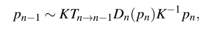
where $p_n$ stands for the pixel on image $I_n$, and $p_{n−1}$ refers to the corresponding pixel of $p_n$ on the image $I_{n−1}$. K is the camera intrinsics matrix, which is known. $D_n(p_n)$ denotes the depth value at pixel $p_n$, and $T_{n→n−1}$ represents the spatial transformation between $I_n$ and $I_{n−1}$. Hence, if $D_n(p_n)$ and $T_{n→n−1}$ are known, the correspondence between the pixels on different images ($I_n$ and $I_{n−1}$) are established by the projection function.
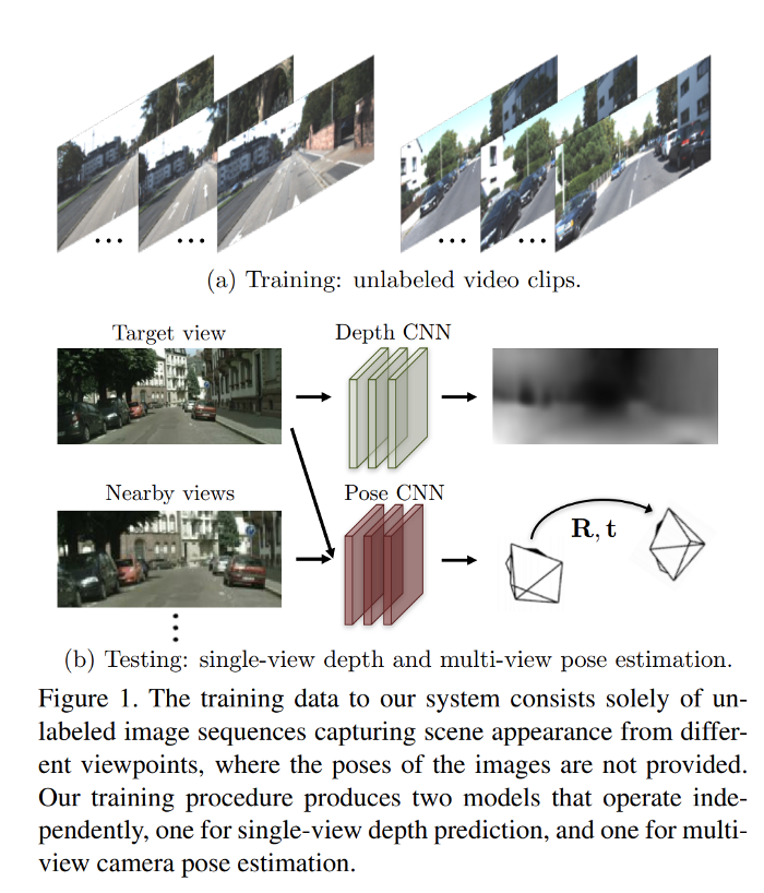
This work tries to estimate the $D$ and $T$ in the above equation by training an end-to-end model in an unsupervised manner to observe sequences of images and to explain its observations by predicting the ego-motion (parameterized as 6-DoF transformation matrices) and the underlying scene structure (parameterized as per-pixel depth maps under a reference view).
They propose two CNNs in this work that are trained jointly: a single-view depth estimation and a camera pose estimation from unlabeled video sequences.
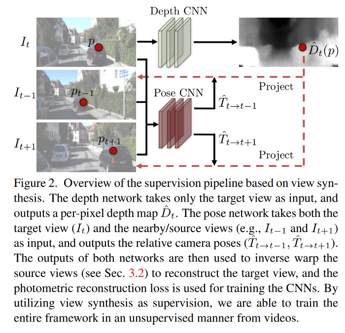
They use the view synthesis idea as the supervision signal for depth and pose prediction CNNs: given one input view of a scene, synthesize a new image of the scene seen from a different camera pose. This synthesis process can be implemented in a fully differentiable manner with CNNs as the geometry and pose estimation modules.
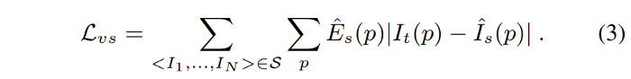
Let’s consider $<I_1, …, I_N>$ as a training image sequence with one of the frames I_t as the target view and the rest as the source views $I_s(1 ≤ s ≤ N, s≠t)$. The view synthesis objective can be formulated as:
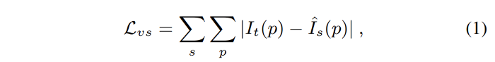
where p indexes over pixel coordinates and $Iˆ_s$ is the source view $I_s$ warped to the target coordinate frame based on a depth image-based rendering module (described in the following), taking the predicted depth $Dˆ_t$, the predicted 4×4 camera transformation matrix $Tˆ_{t→s}$ and the source view I_s as input.
The differentiable depth image-based renderer reconstructs the target view $I_t$ by sampling pixels from a source view $I_s$ based on the predicted depth map $Dˆ_t$ and the relative pose $Tˆ_{t→s}$.
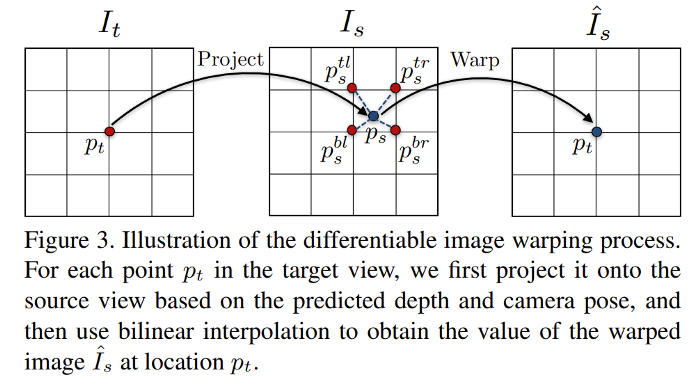
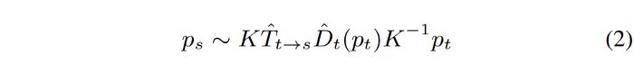
Let $p_t$ denote the homogeneous coordinates of a pixel in the target view, and $K$ denote the camera intrinsics matrix. The $p_t$’s projected coordinates onto the source view $p_s$ (which is a continuous value) can be obtained by:
Then a differentiable bilinear sampling mechanism is used to linearly interpolate the values of the 4-pixel neighbors (top-left, top-right, bottom-left, and bottom-right) of $p_s$ to approximate $I_s(p_s)$.

where $w^{ij}$ is linearly proportional to the spatial proximity between $p_s$ and $p^{ij}_s$, and $sum(w^{ij})=1$.
The above view synthesis formulation implicitly assumes 1) the scene is static without moving objects; 2) there is no occlusion/disocclusion between the target view and the source views; 3) the surface is Lambertian so that the photo-consistency error is meaningful. To improve the robustness of the learning pipeline to these factors, an explainability prediction network (jointly and simultaneously with the depth and pose networks) is trained that outputs a per-pixel soft mask $Eˆ_s$ for each target-source pair, indicating the network’s belief in where direct view synthesis will be successfully modeled for each target pixel.
Since there is no direct supervision for $Eˆ_s$, training with the above loss would result in predicting $Eˆ_s$ to be zero. To prevent this, a regularization term $L_{reg}(Eˆ_s)$ is considered that encourages nonzero predictions.
The other issue is that the gradients are mainly derived from the pixel intensity difference between $I(p_t)$ and the four neighbors of $I(p_s)$, which would inhibit training if the correct $p_s$ (projected using the ground-truth depth and pose) is located in a low-texture region or far from the current estimation. To alleviate this problem, they use an explicit multi-scale and smoothness loss (the $L1$ norm of the second-order gradients for the predicted depth maps) that allows gradients to be derived from larger spatial regions directly.
The final loss function they used for training is as follows:
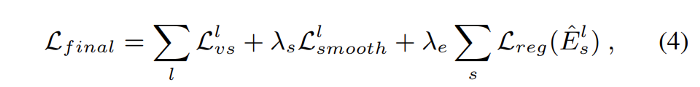
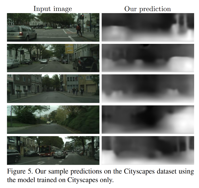
And finally, the results are as follows:
paper: https://arxiv.org/pdf/1704.07813.pdf
code: https://github.com/tinghuiz/SfMLearner
Presentation at NeurIPS 2017:
Digging Into Self-Supervised Monocular Depth Estimation
This paper uses both monocular videos and stereo pairs for depth estimation.
The problem is formulated as the minimization of a photometric reprojection error at training time. The relative pose for each source view $I_t'$, with respect to the target image $I_t$’s pose, is shown as $T_{t→t’}$. Then a dense depth map $D_t$ is predicted in which it minimizes the photometric reprojection error $L_p$:
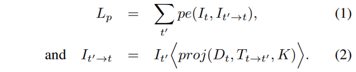
Here $p_e$ is a photometric reconstruction error, e.g. the $L1$ distance in pixel space; $proj()$ is the resulting 2D coordinates of the projected depths $D_t$ in $I_t’$ and $<>$ is the sampling operator. Bilinear sampling is used to sample the source images, which is locally sub-differentiable, and $L1$ and SSIM are used to make the photometric error function $p_e$:
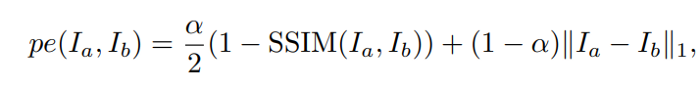
where α = 0.85. They also used edge-aware smoothness:
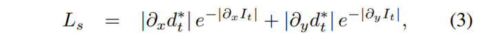
where $d*_t$ is the mean-normalized inverse depth to discourage shrinking of the estimated depth.
In stereo training, the source image $I_t’$ is the second view in the stereo pair to $I_t$, which has a known relative pose. But for monocular sequences, this pose is not known and a neural network is trained jointly with the depth estimation network to minimize $L_p$ and to do pose estimation, $T_{t→t’}$.
For monocular training, two frames temporally adjacent to $I_t$ are used as source frames, i.e. $I_t’ ∈ {I_{t−1}, I_{t+1}}$. In mixed training (MS), $I_t’$ includes the temporally adjacent frames and the opposite stereo view.
The image below shows the overview of the proposed approach and in this paper.
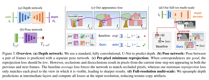
They also propose three architectural and loss innovations which, when combined, lead to large improvements in monocular depth estimation when training with monocular video, stereo pairs, or both:
-
A novel appearance matching loss to address the problem of occluded pixels that occur when using monocular supervision.
-
A novel and simple auto-masking approach to ignore pixels where no relative camera motion is observed in monocular training.
-
A multi-scale appearance matching loss that performs all image sampling at the input resolution, leading to a reduction in depth artifacts
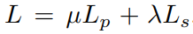
We just explained the main part of the method. To read more about the details of the above innovations, please read the paper. The final loss function is as follows:
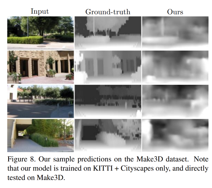
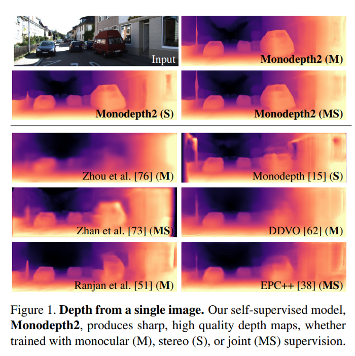
And the results are as follows:
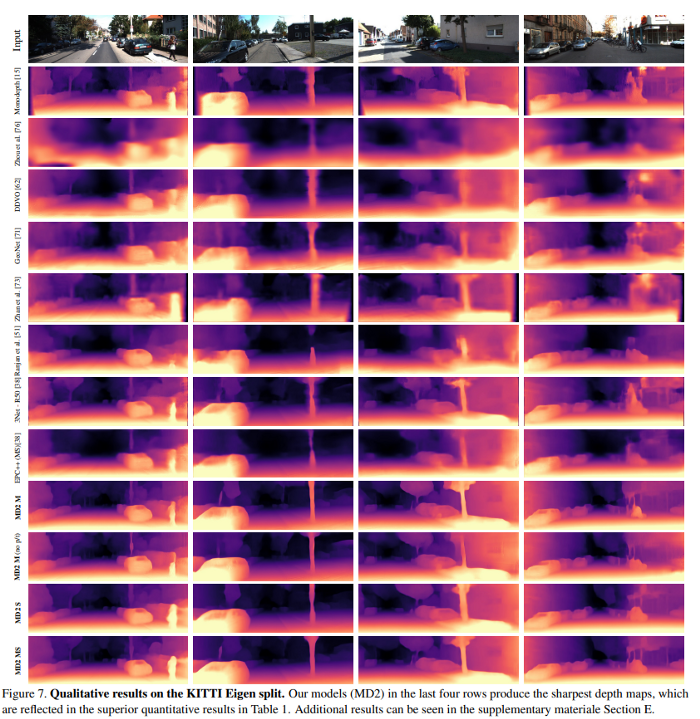
paper: https://arxiv.org/pdf/1806.01260.pdf
code: https://github.com/nianticlabs/monodepth2
video: