Active Learning, Data Selection, Data Auto-Labeling, and Simulation in Autonomous Driving
I will walk through the automatic data collection, data selection, data labeling pipelines, and simulation tools of multiple companies, which I gleaned through numerous speeches and blog posts, as well as review some cutting-edge research articles.


Warning: This blog post is very long. Use the table of content if you want to jump to a specific part:
Deep Learning is going to be in every module of the Self-Driving Car software stack. These deep learning models use data as their learning material, and the quality of the data they are trained on determines their performance. As a result, choosing the optimum training dataset is just as crucial as designing the model itself.
Furthermore, there is always a case with autonomous driving where we don't have data and our model doesn't know what to do. As a result, the models must be trained on as much and diverse data as possible. As a consequence, they'd be equipped to deal with unusual situations in the actual world.
The issue we'd like to look into is that there's a lot of data collected by a fleet of many cars moving around the world, and it's impossible to manually annotate and review all of the data points to find the most useful ones. As a result, we're looking for approaches that assist us to choose or subsample the most informative and valuable data points from live streaming data, such as in self-driving cars, or from unlabeled datasets, and labeling data in an automated and cost-effective manner. In addition, we want to see how we can use simulation environments to generate required data.
In this blog post, I will walk through the automatic data collection, data selection, data labeling pipelines, and simulation tools of multiple companies, which I gleaned through numerous speeches and blog posts, as well as review some cutting-edge research articles. The auto labeling definition is obvious, labeling data using some trained deep learning models (also called pseudo-labeling), but let's see what do we mean by active learning.
Active Learning
Assume that you have an unlabeled dataset and have a budget (money or time) to spend on the labeling task. How can we select and label the most interesting and informative examples from that dataset in which if we train a model on those, it will give us the best possible performance?
The data selection procedure is called Active Learning and the idea is as the following diagram:
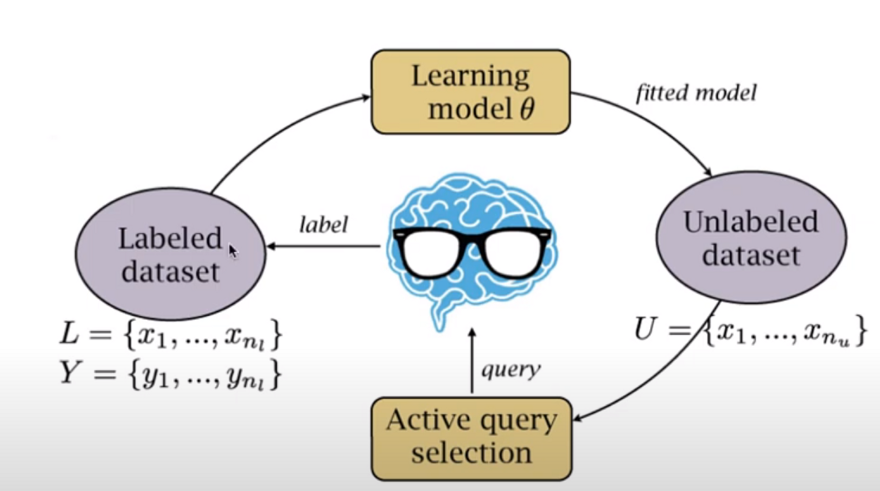
We start with a labeled dataset and use it to train a model. The model is then applied to new unlabeled data points, producing scores based on various metrics for each sample. The data points can then be selected based on the associated scores. After that, a human annotator will annotate these selected samples and add them to the labeled dataset. The model will then be trained on that dataset once more, and the procedure will be repeated until the results are satisfactory.
Some resources consider the following main categories for active learning techniques: diversity-based sampling, and uncertainty-based sampling:
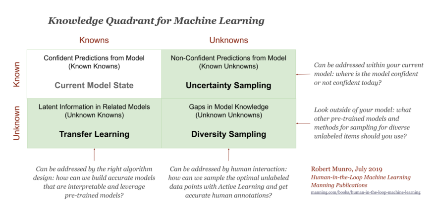
The right column above represents Active Learning: the Known Unknowns that can be addressed with Uncertainty Sampling and the Unknown Unknowns that can be addressed with Diversity Sampling. Some examples of the two mentioned categories can be found here and here.
Here I list some of the techniques I found which can fall into one or multiple mentioned categories. Let's check some of them (mostly from this lecture):
Random Sampling: One way to select some samples from the dataset is to do random sampling. But there is no guarantee that selected samples are informative enough or maybe they are similar to each other.
Metadata-based Sampling: The metadata distribution of the dataset refers to parameters that describe the image's content (such as luminance and color channels) or the conditions in which the image was captured (time, temperature, and location). The primary task is to determine what the dataset should ideally represent in these proportions. One sampling technique for data selection is data querying based on metadata information.
Diversity-based sampling: Diversity-based sampling, which is based on the distance between samples in embedding space, is a more comprehensive and efficient method of data selection. Its goal is to select a diverse dataset that covers all possible scenarios, ensuring that the model is trained even on edge or corner cases. By using a diverse training subset, redundant samples and over-represented data that can lead to overfitting are removed, improving model accuracy. It should be noted that some of the other approaches mentioned here may also fall into this or other categories. For example, the following method, which employs an ensemble of models, can be used to assess the diversity of a new data point.
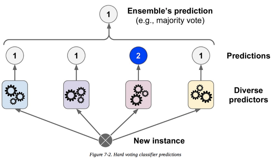
Ensemble of models: Using an ensemble of trained models and then feeding the data point into all of them and voting on their outputs is one technique to choose a data point. If the models agree on the outcome, it means the data point is similar to the data used to train the model and is hence uninformative. If models disagree on the data, it implies that the models lack sufficient information about the sample, and there is something to be learned from this data point.
Entropy: The other approach is to use Entropy, which shows the uncertainty, as a score for selecting samples. For example, for a classification task, the entropy for the distribution over different classes can be calculated. If the probability for one class is much higher than others, the calculated entropy would be low which means the model is certain about that sample. And if the probabilities for all classes or several classes are almost the same, the calculated entropy would be high and this shows the model is uncertain about the data point and it will be selected to be labeled. To summarize, the idea behind uncertainty-based sampling is that algorithms ensure that data, where the model is uncertain, is added to the training set.
Ensemble + Entropy: It is also possible to combine the two mentioned approaches. First, use an ensemble of models to get outputs (distribution over different classes for classification task for example) and then combine the outputs (take the mean of those distributions for example) and then calculate the entropy for the resulting distribution.
Monte Carlo Dropout: The other technique is to use Monte Carlo Dropout. The idea is to train a model with dropout but does not turn the dropout off in the inference phase. Then feeding the data point into the model with dropout several times. It would be somehow similar to the ensemble idea but just needs to train one neural network. The entropy idea can be used here too similar to the previous case.
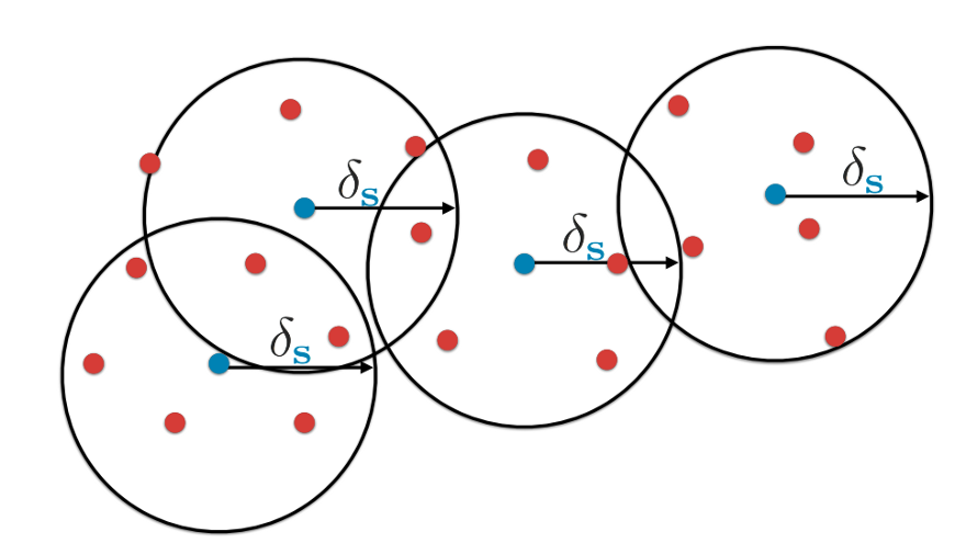
Geometric Approach or Core-Set: The idea is to pick a small set of points (blue points) whose neighbors (red points) are within a certain distance of these blue points so that if we train a model on these blue points (selected points), the model's performance will be as close to that of a model trained on the entire dataset as possible (all blue and red data points). They define a loss function to select these data points that you can check the paper for more detail. It is also possible to use clustering algorithms to find clusters and select the centroid of the cluster as the blue point.
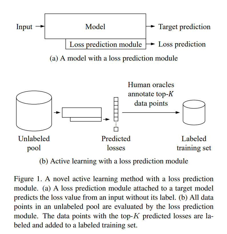
Learning the Loss: the idea is to train the model to predict the cross-entropy loss as an output. So during the training phase, we can teach the model to do the loss prediction and use it on unlabeled data points. Then, the predicted loss can be used as a score for each data point to be selected for labeling or not.
Consistency-based sampling: Entropy-based and consistency-based methods are complementary. Entropy-based methods perform well on samples coming from easy classes (classes that the model performs well in general but not for some cases) and not very well on hard classes (classes that the model does not perform well in general). As a result, active learning using uncertainty improves the performance over the classes that the model works already well. But for hard classes, the scores by the uncertainty methods are not reliable. Here is an example from a paper called "Not All Labels Are Equal":
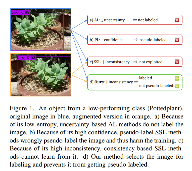
The other problem with uncertainty-based methods is that by focusing only on the samples that the model is uncertain about, the selected samples will be just the hard samples which will have a different distribution than the main data and the task we want the model to perform on.
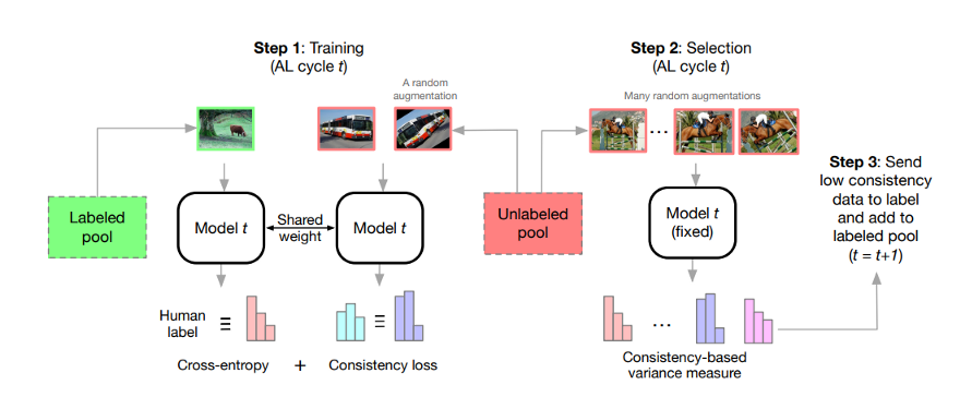
On the other hand, consistency-based methods perform well on samples coming from hard classes. The idea in consistency-based methods is that during training, both labeled and unlabeled data are used for model optimization, with cross-entropy loss encouraging correct predictions for labeled samples and consistency-based loss encouraging consistent outputs between unlabeled samples and their augmentations. During sample selection, the unlabeled samples and their augmentations are evaluated by the model developed during the training stage. The consistency-based metric is used to evaluate their outputs. Samples with low consistency scores are chosen for labeling and sent to the labeled pool. Here is an illustration of the proposed framework at t_th active learning cycle in a paper called "Consistency-based Semi-supervised Active Learning":
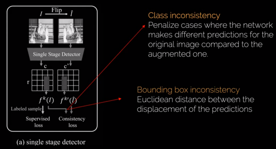
Combining uncertainty and consistency methods (e.g. multiplying the scores) can improve the performance over both. The paper called "Not All Labels Are Equal" proposes a unified strategy to choose which samples to manually label and which samples can be automatically labeled. They consider the object detection task in their paper and try to build a more general acquisition function to score data points which is not only based on entropy but also based on consistency. The idea is to use again both labeled and unlabeled data and pass them through the detector. There are two losses in their method: one is the supervised loss for labeled data and the other one is the consistency loss which is for both labeled and unlabeled data. Then they have the scoring function, which will select which samples go to the human annotators, and also which samples are easy samples and need to go for the pseudo labeling. So the valuable time of the annotator will not be spent on easy samples. Here is the diagram of their proposed method:
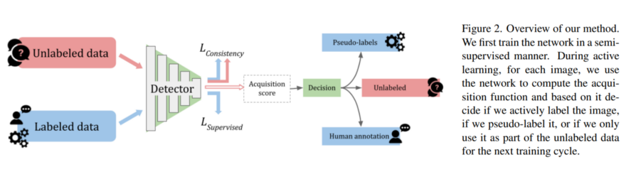
For the consistency loss, they have two terms: one for class inconsistency and one for bounding box inconsistency.
There is a lot more to say about active learning, but we'll stop here. Now, let's look at what big companies do in the real world.
NVIDIA
NVIDIA proposes to use pool-based active learning and an acquisition function based on a disagreement between several trained models (the core of their system is an ensemble of object detectors providing potential bounding boxes and probabilities for each class of interest) to select the frames which are most informative to the model. Here are the steps in their proposed approach:
-
Train: Train N models initialized with different random parameters on all currently labeled training data.
-
Query: Select examples from the unlabeled pool using the acquisition function.
-
Annotate: Annotate selected data by a human annotator.
-
Append: Append newly labeled data to training data.
-
Go back to 1.

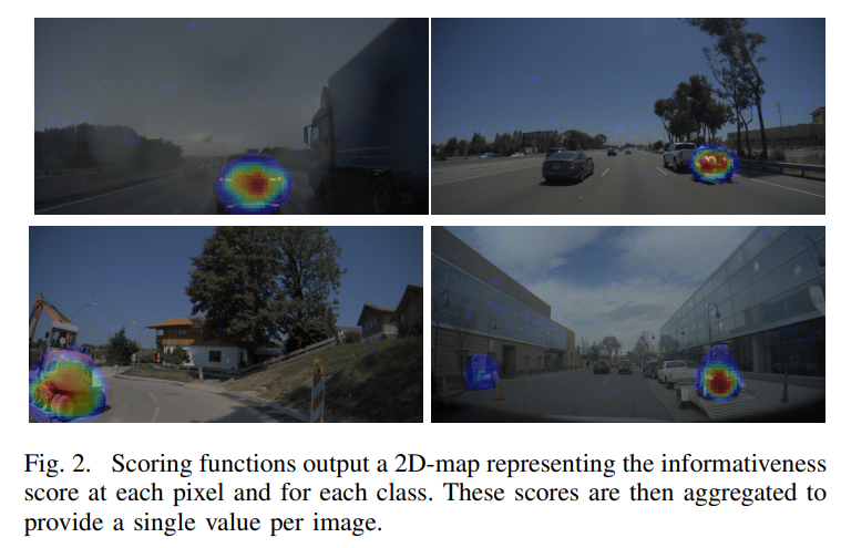
They assume the object detector generates a 2D probability map for each class (bicycle, person, car, etc.). Each position in this map relates to a pixel patch in the input image, and the probability indicates whether an object of that class has a bounding box centered there. This type of output map is commonly found in one-stage object detectors like SSD or YOLO. They use the following scoring functions:
- Entropy: They compute the entropy of the Bernoulli random variable at each position in the probability map of a specific class:

where p_c represents probability at position p for class c.
- Mutual Information (MI): This method makes use of an ensemble E of models to measure disagreement. First, the average probability over all ensemble members for each position p and class c is computed as:
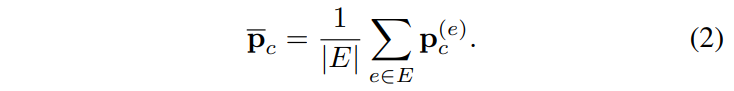
where |E| is the cardinality of E. Then, the mutual information is computed as:
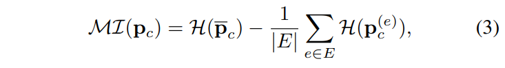
MI encourages the selection of uncertain samples with high disagreement among ensemble models during the data acquisition process.
-
Gradient of the output layer (Grad): This function computes the model's uncertainty based on the magnitude of "hallucinated" gradients. The predicted label is specifically assumed to be the ground-truth label. The gradient for this label can then be calculated, and its magnitude can be used as a proxy for uncertainty. Small gradients will be produced by samples with low uncertainty. Then a single score based on the maximum or mean variance of the gradient vectors is assigned to each image.
-
Bounding boxes with confidence (Det-Ent): The predicted bounding boxes of the detector have an associated probability. This allows computing the uncertainty in the form of entropy for each bounding box.
To aggregate the scores obtained via the mentioned techniques above, two approaches can be used: taking the maximum or the average. Taking the maximum can lead to outliers (because the probability at a single position determines the final score), whereas taking the average favors images with a high number of objects (since an image with a single high uncertainty object might get a lower score than an image with many low uncertainty objects). For the maximum, the score is defined as follows:

Then the top N images with the highest scores can be selected to be annotated by human annotators. It is also possible to first calculate a feature vector for each image using for example a CNN network, and then using some techniques using k-means++, Core-set, or sparse-modeling (OMP), which combines diversity and uncertainty, to select samples.
Here is a short video of the performance of their approach:
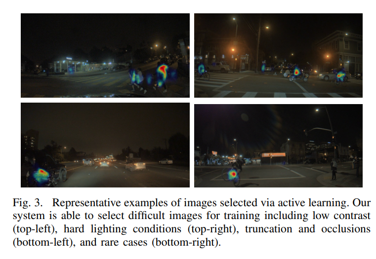
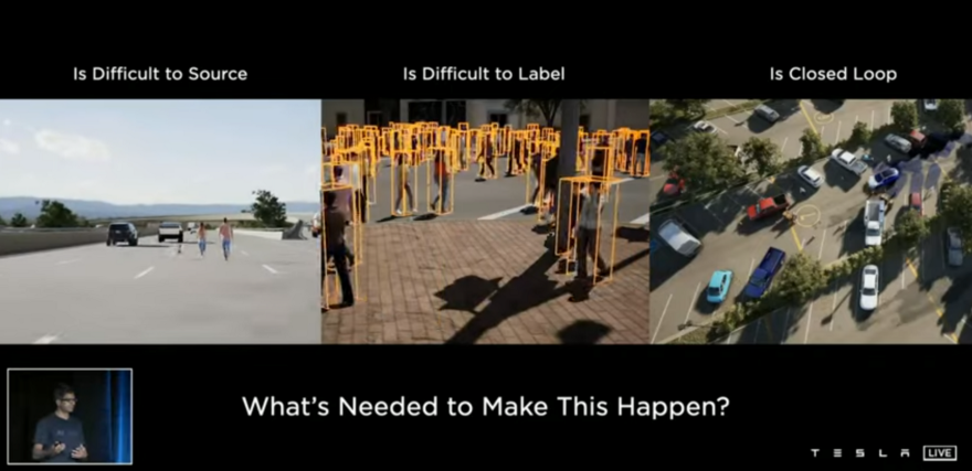
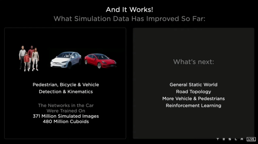
In addition to the mentioned active learning approach, NVIDIA has developed another solution to deal with the challenges of data collection and labeling. They discussed this challenge at CES2022, stating that the most interesting data that we are interested in labeling is also the most challenging. Here are some examples of dark, blurry, or hazy scenes.
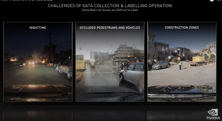
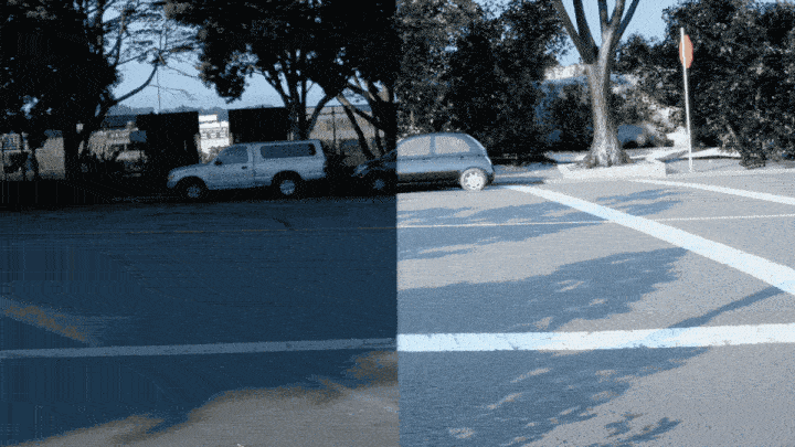
There are also scenes that are difficult to comprehend, such as occluded vehicles or pedestrians. Moreover, there are some scenes not often seen, like construction zones. Due to these issues, autonomous vehicle developers need a mix of real and synthetic data. NVIDIA built DRIVE Sim replicator to deal with all of these labeling challenges. DRIVE Sim is a simulation tool built on Omniverse that takes advantage of the platform's features. Engineers can generate hard-to-label ground truth data from this replicator and use them to train deep neural networks that make up autonomous vehicle perception systems. As a result of synthetic data, developers have more control over data development, allowing them to tailor it to their specific needs and collect the data they want even before any real-world data collection for those situations.
As collecting and labeling real-world data is difficult, taking synthetic data and augmenting it with real-world data removes this bottleneck, allowing engineers to take a data-driven approach to develop autonomous driving systems. This improves real-world results and significantly speeds up AV development.
Another problem is the gap between the simulator world and the real world. The gap may be pixel-level or content-level. Omniverse Replicator is designed to narrow the appearance and content gaps. Read more about the capabilities of this amazing simulator here.
Waymo
Waymo uses active learning too, obviously. In this talk, Drago Anguelov explains about the ML factory used at Waymo:
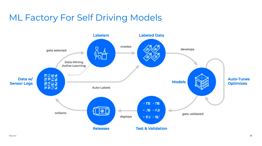
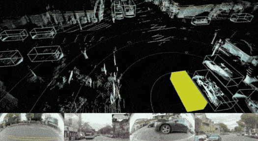
The lifecycle is almost similar to what we saw for NVIDIA. Most of the data come from some common scenarios and does not have enough information for the model to learn. So it is essential to know how to select the data. They have data mining and active learning pipelines to find rare cases and situations where the models are uncertain or inconsistent over time and label those cases. Then this labeled data will go for model training. They also have auto-labels in their system. When you collect data, you also see the future for many objects. This knowledge about the past and the future will help annotate data better, go back to the model that does not know the future, and replicate it with the model.
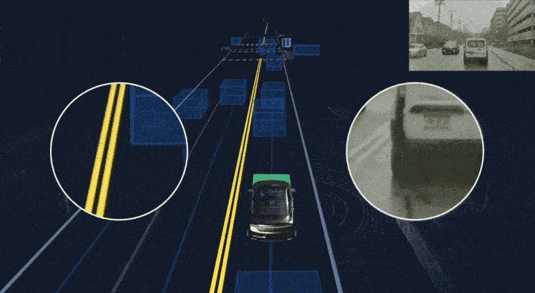
Waymo also released the Open Motion Dataset and had a competition at CVPR 2021. The dataset is labeled using a deep learning model in offline mode published in CVPR 2021: Offboard 3D Object Detection from Point Cloud Sequences. Running the model in offline mode is not limited by latency constraints on the vehicle and also benefits from seeing the future, as it has access to the full scene and can go backward and forward in time. This labeling approach in offline mode can be used to label a lot of data and then train deep learning models on that data.
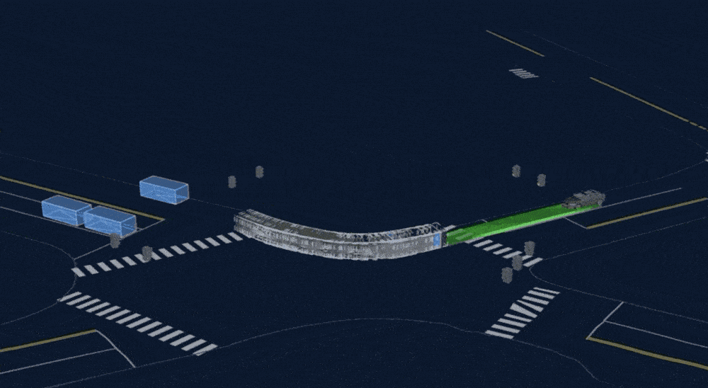
The offboard 3D object detection paper presents new techniques for automatically labeling the point clouds created by lidar sensors. Taking advantage of the fact that different image frames capture complementary views of the same object, this team has developed a labeling system that includes multi-frame object detection over time. Here is their 3D auto-labeling pipeline (the pipeline is explained in the image caption):
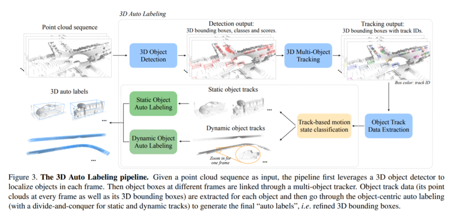
The 3D Auto Labeling pipeline. Given a point cloud sequence as input, the pipeline first leverages a 3D object detector to localize objects in each frame. Then object boxes at different frames are linked through a multi-object tracker. Object track data (its point clouds at every frame as well as its 3D bounding boxes) are extracted for each object and then go through the object-centric auto labeling (with a divide-and-conquer for static and dynamic tracks) to generate the final "auto labels", i.e. refined 3D bounding boxes.*
And here is its performance compared to state-of-the-art: source
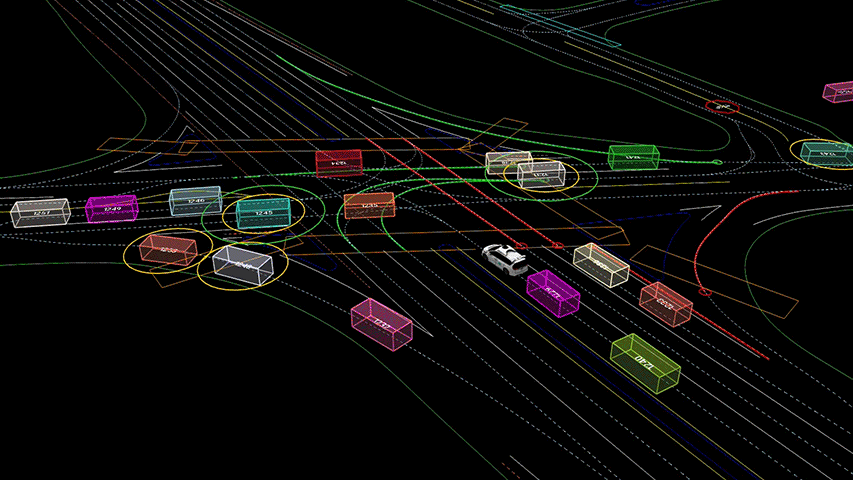
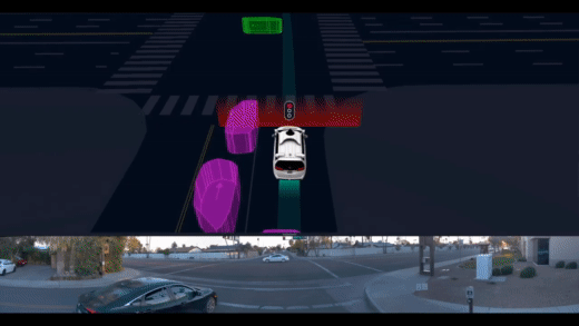
Waymo, like NVIDIA, has a simulator called SimulationCity. The goal is to gain a better understanding of how the Waymo Driver responds to the full range of behaviors that it will encounter in the real world.
Assume we simulate a scenario of tailgating at an intersection. To evaluate the Waymo Driver's behavior, we want to understand as many possible outcomes as possible and their likelihood of occurring. If we chose a random tailgating scenario, the tailgater would almost certainly brake in time. However, it is critical to assess how the Waymo Driver behaves when the tailgater fails to brake in time, for example, when the tailgater is distracted or inattentive. As more variations of the same scenario are simulated, we observe a convergence of the distribution of outcomes between what we observe in simulation and the real world. Additionally, SimulationCity enables us to investigate rare events in order to create risky scenarios that the Driver has never encountered before, but that have been proven to be both realistic and extremely useful.
Having a large and high-quality dataset, as well as the simulation required to generate the required data, is critical for deep learning models and autonomous driving to operate safely and handle rare cases such as the following:
This scenario depicts a car passing a red traffic light and entering an intersection when the green light is for the ego car, but the vehicle is capable of handling the situation and yielding to the crazy car before proceeding. This demonstrates that Waymo is performing an excellent job of data collection, data selection, and corner case analysis, as well as simulation, to train their models.
Tesla
In this talk on Tesla AI Day in 2019, Andrej Karpathy explains the active learning procedure at Tesla, which they call the Data Engine. For example, in an object detection task and for a bike attached to the back of a car, the neural network should detect just one object (car) for downstream tasks such as decision-making and planning. Check the following image:
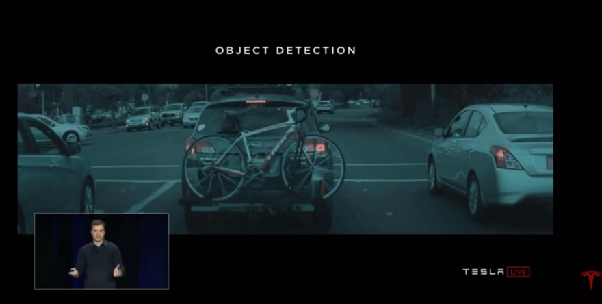
They find a few images that show this pattern and use a machine learning mechanism to search for similar examples in their fleet to fix this problem. The returned images from the fleet can be as follows:
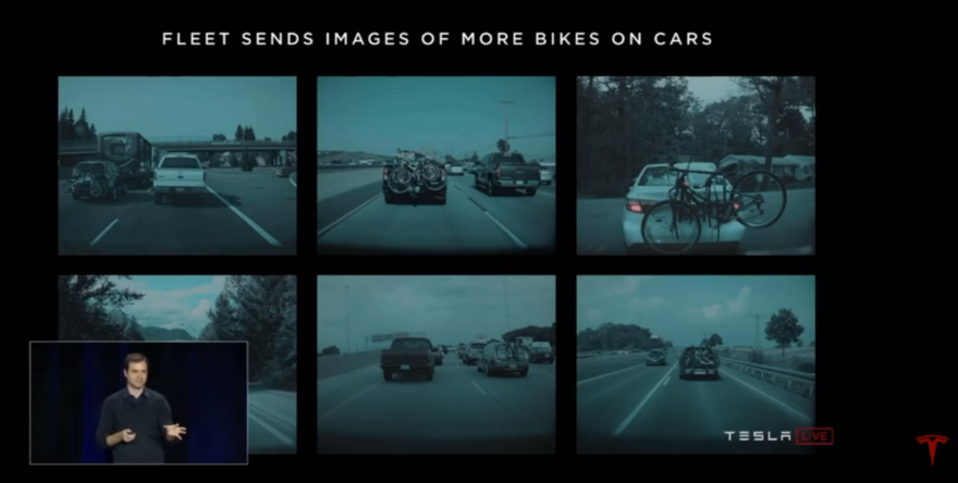
Then human annotators will annotate these examples as single cars, and the neural network will be trained on these new examples. So, in the future, the object detector will understand that it is just an attached bike to a car and consider that as just a single car. They do this all the time for all the rare cases. So their model will become more and more accurate over time.
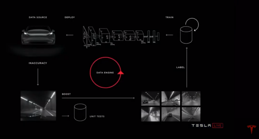
After collecting some initial data, the models are trained. Then, wherever the model is uncertain, or there is human intervention or disagreement between the human behavior and the model output, which is running in shadow mode, the data will be selected to be annotated by humans, and the model will be trained on that data. For example, if the model for lane line detection does not work very well in tunnels, they will notice a problem in tunnels. So they use the explained mechanism to find similar images, annotate those, and train the model on those.
Andrej also talks about their automated mechanism to do data labeling in addition to expensive human annotators, called Fleet Learning.
As an example, he talks about automatic cut-in detection. You drive on a highway in a lane, and someone from the left or right lane cuts into your lane. Their fleet is capable of detecting this scenario.
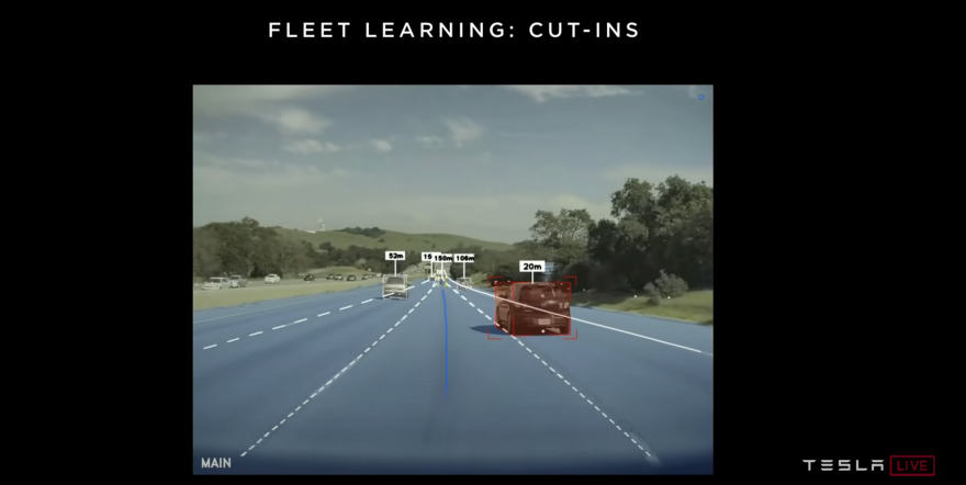
This is not a hard-coded procedure to write rules or codes to identify this event. It is a learning process. They ask the fleet to find scenarios where a car from the left or right lane transitions to the ego lane. Then they go backward in time and automatically annotate that scenario and train neural networks on it. So the neural network will pick up many of these patterns and learn from them. As Andrej says, the neural network may also learn about the left or right blinkers, which show lane change internally from these examples without any hard-coding. After the whole training procedure, they can deploy the model in shadow mode. So, in shadow mode, the network always makes predictions about the events and acts as a trigger to find mispredictions. These false positives and false negatives detected freely by the cut-in network will be added to the training dataset and go into the explained Data Engine and training procedure. After several rounds of the same process for the cut-in network, and when they are happy with the performance, the trained model can be turned on and take control of the car instead of being in shadow mode.
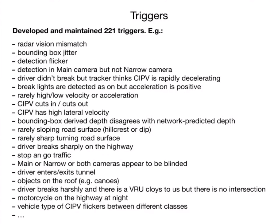
Here are some of the triggers they use:
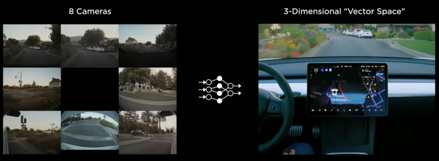
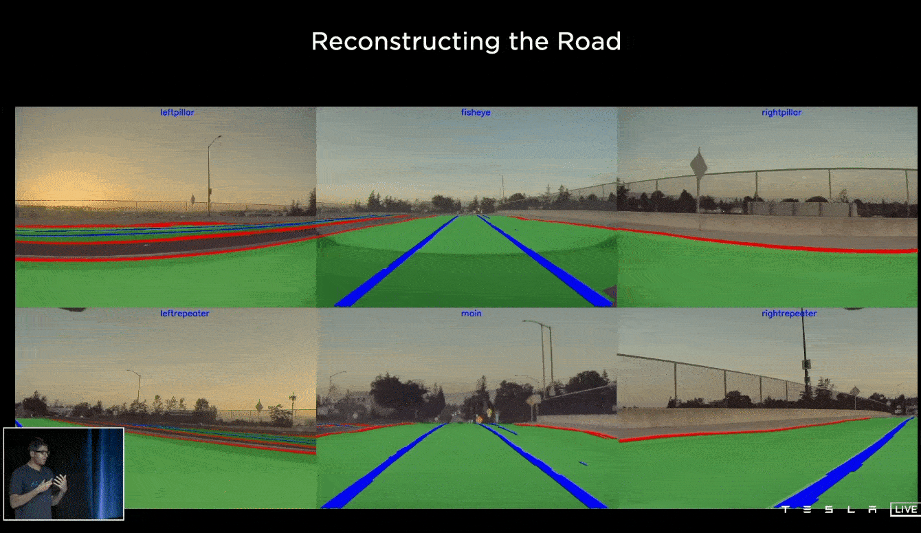
On Tesla AI day in 2021, they discuss the Autopilot software stack in more detail. They also talk about data collection and auto-labeling. Andrej talks about collecting clean and diverse data for training neural networks. Instead of image space, they go for vector space, a 3D representation of everything you need for driving. It is the 3D position of lines, edges, curbs, traffic signs, traffic lights, cars, their positions, orientations, depth, velocity, etc. It gets raw image data and outputs the vector space for the scene. Part of the vector space is shown on the Tesla car screen in the following image:
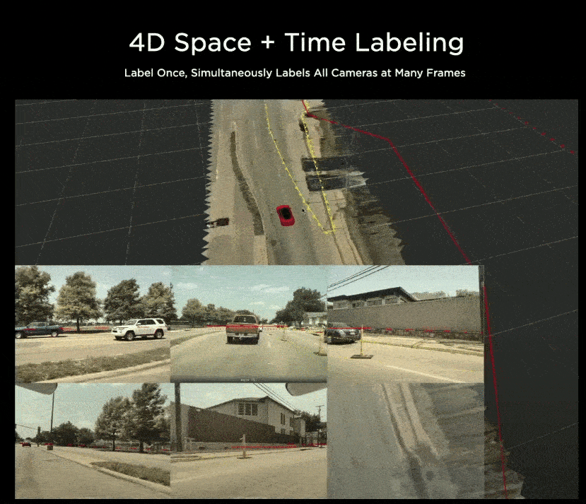
Andrej also talks about data labeling in vector space instead of image space. The human annotator labels data in the 3D vector space, and it will be projected into image space automatically as shown in the GIF below:
But even this improved labeling procedure is not scalable. Active learning and auto-labeling can help here. Here is an example of how they label a clip. It has data from different sensors, such as cameras, IMUs, GPS, etc., and can last from 45 seconds to 1 minute.
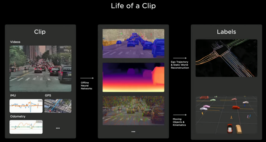
Tesla engineering cars or customer cars can upload the clips to Tesla servers. Following this, many neural networks are run in offline mode to produce intermediate results, such as segmentation masks, depth, and point matching. Then a lot of robotics and AI algorithms are then utilized to create the final set of labels needed to train the neural networks.
Road surface labeling (segmentation) is one of the tasks they discuss. Typically, we can represent a road surface with splines or meshes, but due to topological restrictions, they are not differentiable and not appropriate for deep learning. Also, segmenting in each image space and for each camera view and then joining them together to represent the scene does not work very well. Instead, they use Neural Radiance Fields or NeRF and an implicit representation to represent the road surface (I LOVED this idea). You can check this, this, and this to learn more about NeRF.
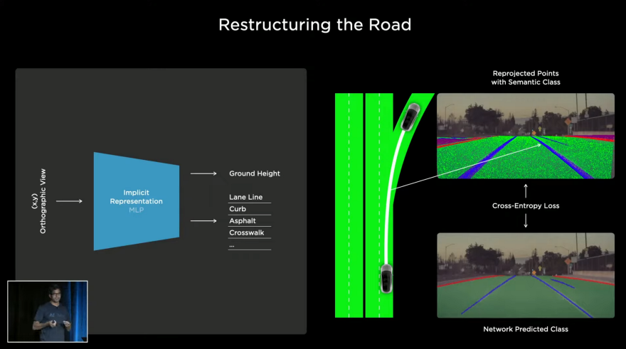
Then they can query an (x, y) point on the ground, and the network can predict the height of the ground surface and the semantic class for that point, such as lane line, curb, asphalt, crosswalk, etc. By having the input (x, y) and the predicted height (z), we will have a 3D point that can be projected to all camera views. Making millions of these queries and projecting the resulting 3D point into all camera views can achieve semantic segmentation, such as the top-right picture in the above image. Then the resulting images from all camera views can be compared to the semantic segmentation results from image space and by a joint optimization for all camera views across space and time can produce an excellent reconstruction:
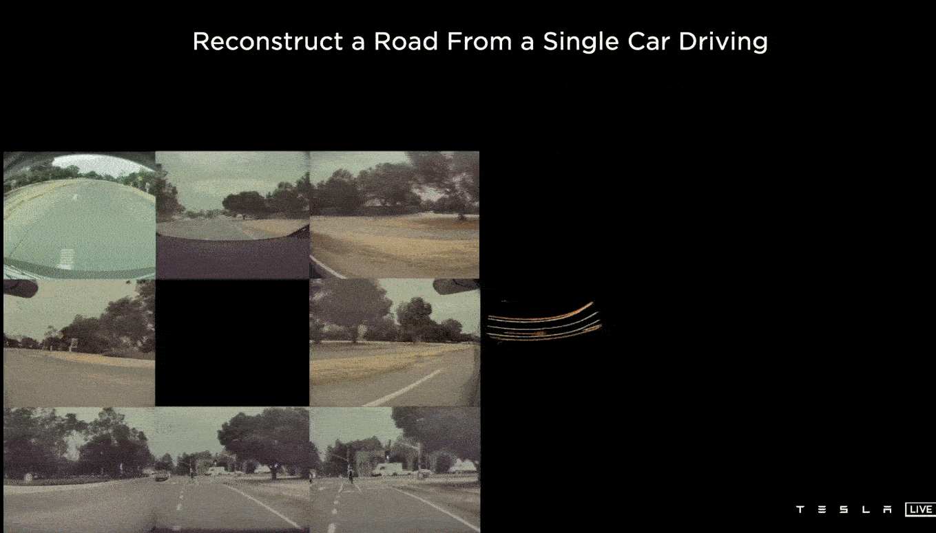
Each car that drives on some roads does the labeling. By collecting this labeled data from one or many cars in the same area, they can bring them all together and align them using various features such as road edges, lane lines, etc., which all agree with each other and also with the image space observations and can generate the whole scene. This produces an effective way of labeling the road surface. After the labeling process, human annotators can check them and clean up any noise in the data, or maybe add metadata to that to make it even more prosperous.
They also talk about more data collection such as static objects, walls, barriers, etc. We don't go into more details here but you got the idea.
In addition to the auto-labeling procedure, explained above, Tesla has a simulator too and uses it for data generation and labeling. Here is their talk at Tesla AI Day 2021:
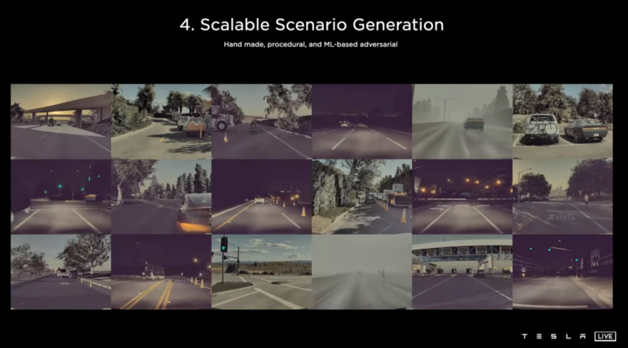
They mention that using their vector space, they can produce the scenes they want very quickly! The simulator can be used in different cases:
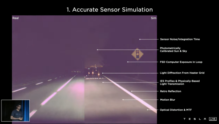
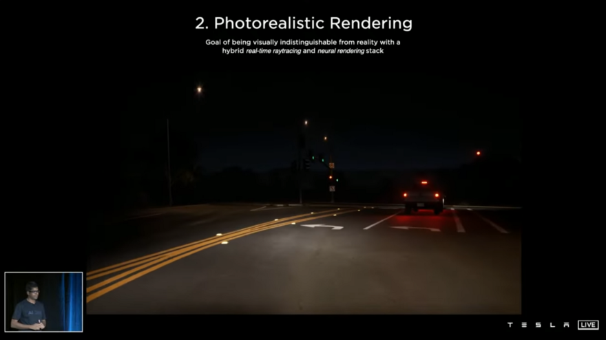
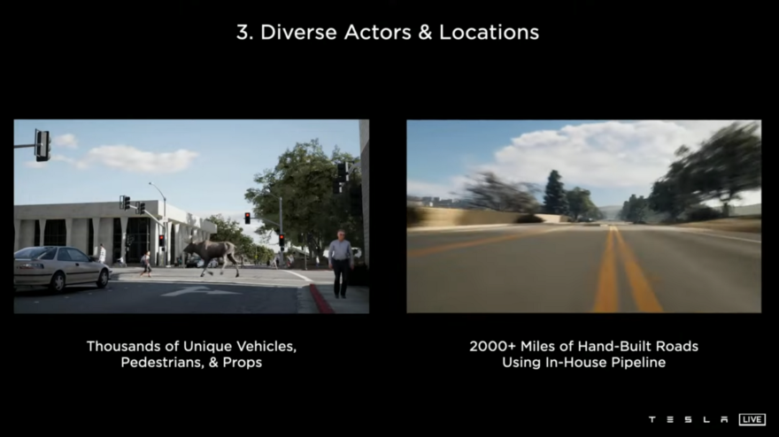
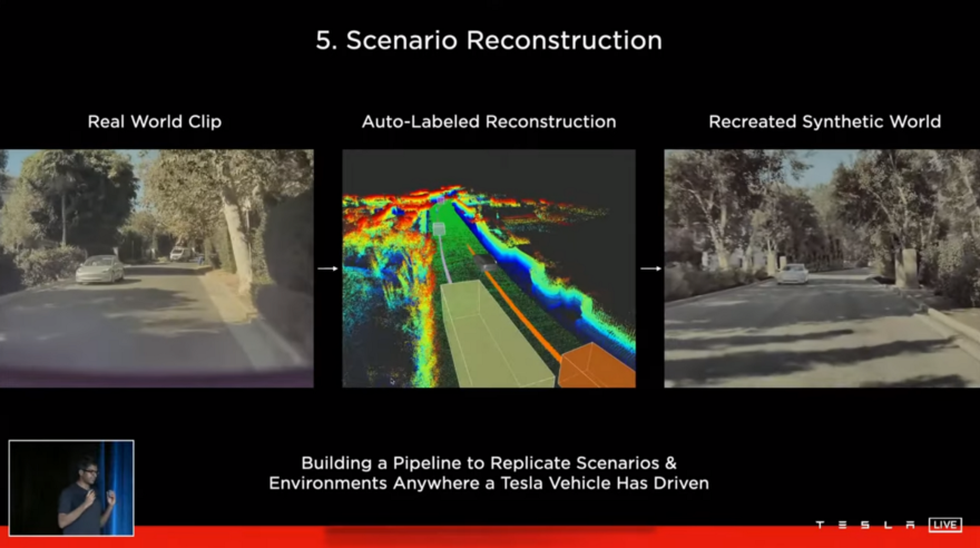
To have such a good simulator, it needs accurate sensor simulation, photorealistic rendering, Diverse actors and locations, scalable scenario generation, real-world scenario reconstruction.
They also mentioned doing Reinforcement Learning using their simulator, which is my favorite topic and I'm doing my Ph.D. on that.
I think that's enough for Tesla. Let's go for another company.
Cruise
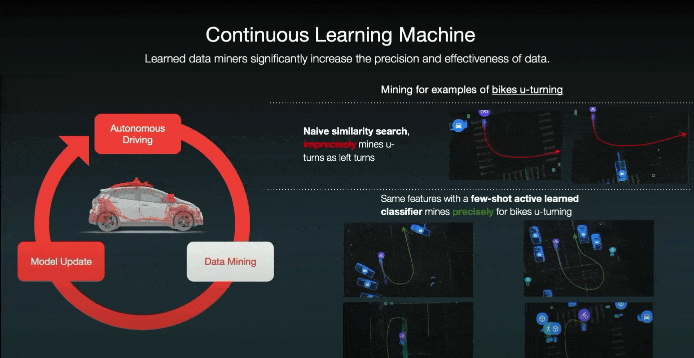
Cruise also makes use of active learning. They refer to it as the Continuous Learning Machine (CLM).
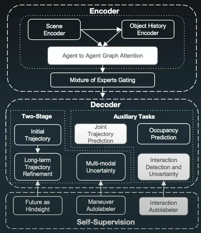
Consider the task of prediction. The motion prediction model must be capable of handling both the nominal and longtail cases well. Here is the end-to-end motion prediction model which Cruise uses and announced in the Cruise Under the Hood event recently:
It is critical to note that while these longtail events do occur in the data collected on the road, they are extremely rare and infrequent. As a result, we concentrate on identifying the needle in the haystack of daily driving and use upsampling to teach the models about these events.
A naive approach to identifying rare events would be to manually engineer "detectors" for each of these longtail situations to assist in data sampling. For instance, we could create a "u-turn" detector that generates sample scenarios whenever it is triggered. This approach would enable us to collect targeted data, but quickly fails when scaling up, as it is impossible to write a detector that is sufficiently specific for each unique longtail situation.
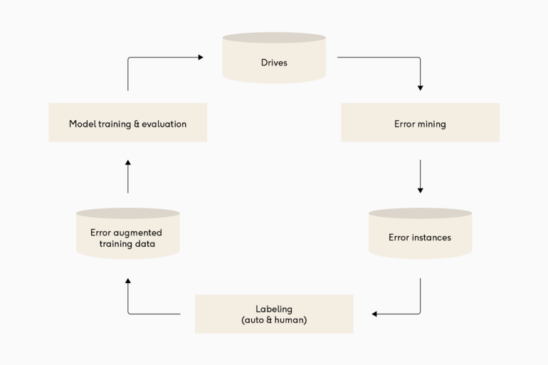
Self-supervised learning is a viable option for the prediction task at hand. In each scenario, we can compare our model's prediction to the ground truth future trajectory of each car, and if they differ, we can label that scenario and train our model on that. These error situations can be automatically identified and mined. The labeling does not require human annotations and can be done automatically using the logged future trajectory of the car. Following that, these longtail events should be upsampled. The auto-labeled approach ensures maximum coverage of the dataset by identifying and mining all model errors, ensuring that no valuable data is missed. Additionally, it keeps the dataset as lean as possible by ensuring that no additional data for already-solved scenarios is added to the dataset.
-
Drives: The CLM starts with the fleet navigating in the city.
-
Error Mining: Active learning is used to automatically identify error cases, and only scenarios with a significant difference between prediction and reality are added to the dataset. This enables highly targeted data mining, ensuring that we add only valuable data and avoid bloating the datasets with easy and uninformative scenarios.
-
Labeling: All of our data is automatically labeled by the self-supervised framework, which uses future perception output as the ground truth for all prediction scenarios. While the core CLM structure is applicable to other machine learning problems where a human annotator is required, fully automating this step within prediction enables significant scale, cost, and speed improvements, allowing this approach to span the entire longtail.
-
Model Training and Evaluation: The final step is to train a new model, run it to rigorous testing, and finally deploy it to the road. The testing and metrics pipelines ensure that a new model outperforms its predecessor and generalizes well to the nearly infinite variety of scenarios found in the test suites. Cruise has made significant investments in the machine learning infrastructure, which enables the automation of a variety of time-consuming tasks. As a result, they are capable of creating an entire CLM loop without human intervention.
Let's review some examples.
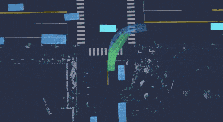
U-turn is one of the longtail scenarios which happens very rarely. The following image shows different trajectories (red ones) in an intersection starting from the black point.
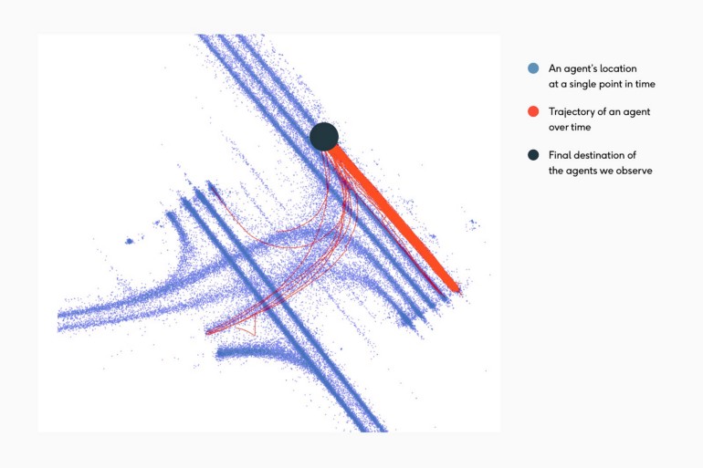
As demonstrated in the image, the majority of the dataset consists of drivers traveling straight with few left turns, even fewer lane changes, and only two U-turn trajectories. Another example of the uncommon mid-block u-turn can be seen below:
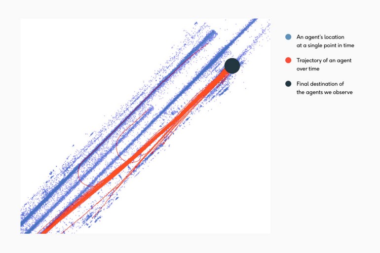
When CLM principles are applied, the initial deployment of the model may underpredict U-turn situations. As a result, when we sample data, we frequently encounter error situations involving U-turns. Over time, the dataset gradually increases its representation of U-turns until the model is capable of sufficiently predicting them and the AV is capable of accurately navigating these scenarios.
K-turn is the other longtail scenario. The K-turn is a three-point maneuver that requires the driver to move forward and backward in order to complete the turn in the opposite direction. These are uncommon and are most frequently used when the street is too narrow for a U-turn.
Cut-in is another rare scenario that we need to be able to predict in order to handle the situation and yield for the car if needed.
Another kind of interesting scenario is the one with the interaction between agents. For example:
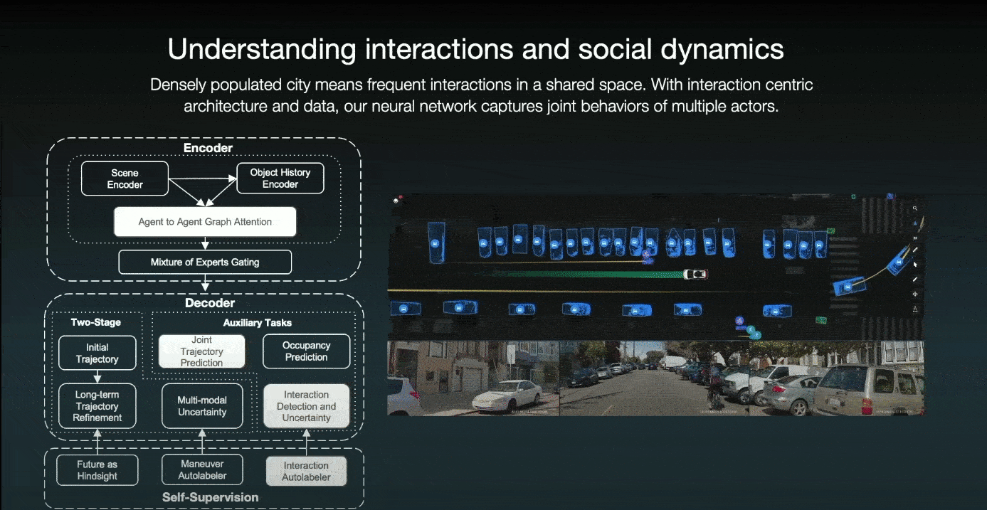
Cruise employs an interaction-centric architecture with an agent-to-agent graph and an attention mechanism for detecting agent interaction. For instance, in the previous scenario, the ego car and a bicycle are driving alongside one another, and the parked car wants to slightly come back. The car understands the interaction and anticipates that the cyclist will nudge to the left to avoid it. As a result, the self-driving car slows and yields to the cyclist.
Additionally, they have an interaction auto-labeler that can determine whether or not a pair of agents interacts. And, if that is the case, who wins the interaction? Then, as additional self-supervision, this interaction auto-labeler can mine scenarios and define auxiliary tasks for interaction detection and resolution.
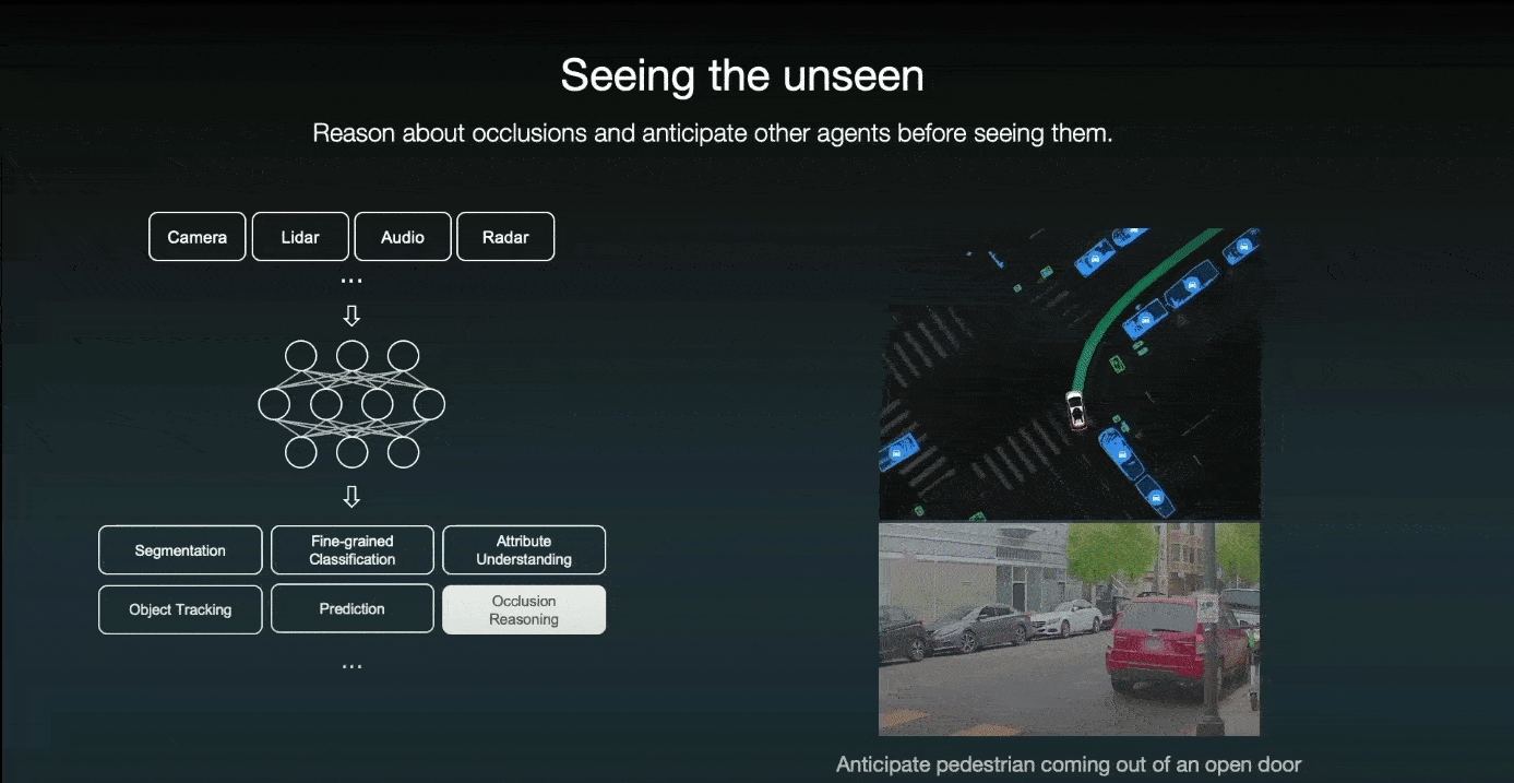
Not only the future is uncertain, but also the world behind occlusions. Therefore, they designed their AI system to understand which part of the world is occluded and proactively anticipate other agents before even seeing them. For example, when a door pops open, their system can anticipate a pedestrian coming out of the door. So the car slows down immediately and steers further away from it.
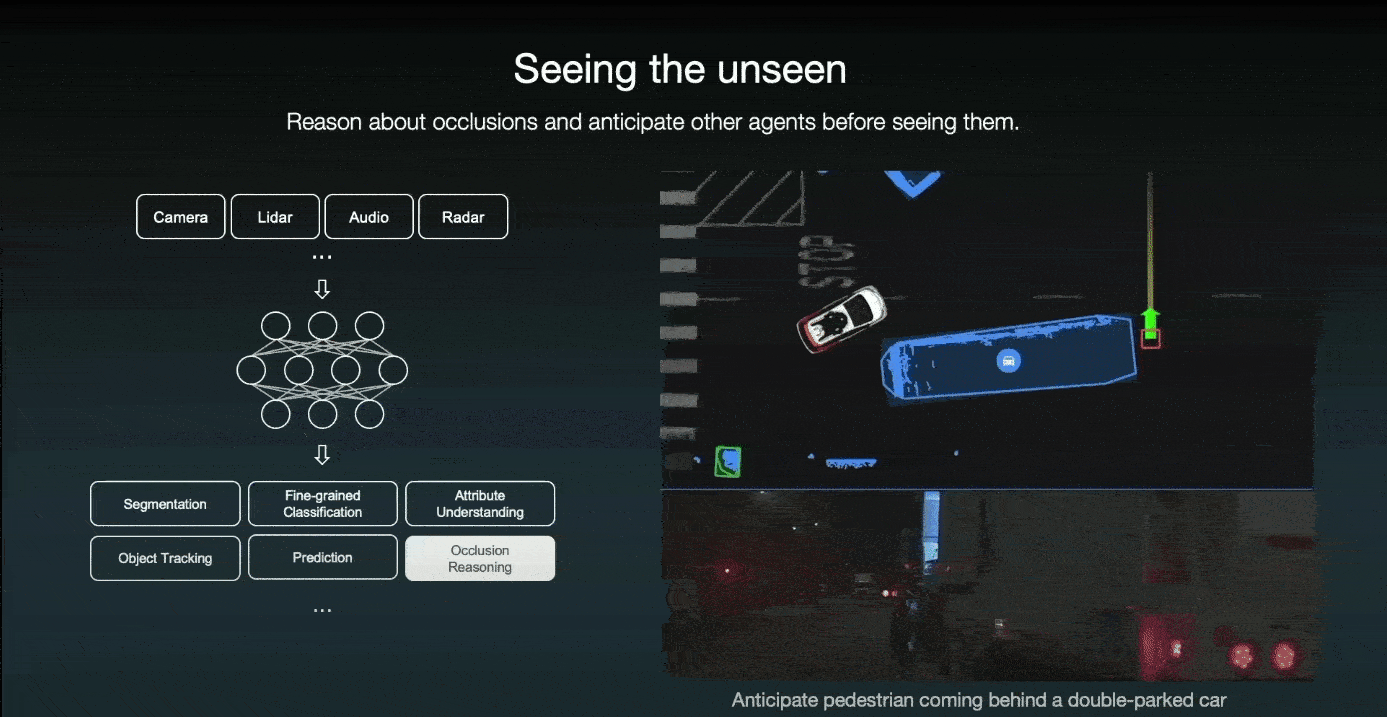
The other example is when a large garbage truck obscures the driver's view; even though the driver cannot see anything behind the truck, the system imagines a pedestrian attempting to cross the street.
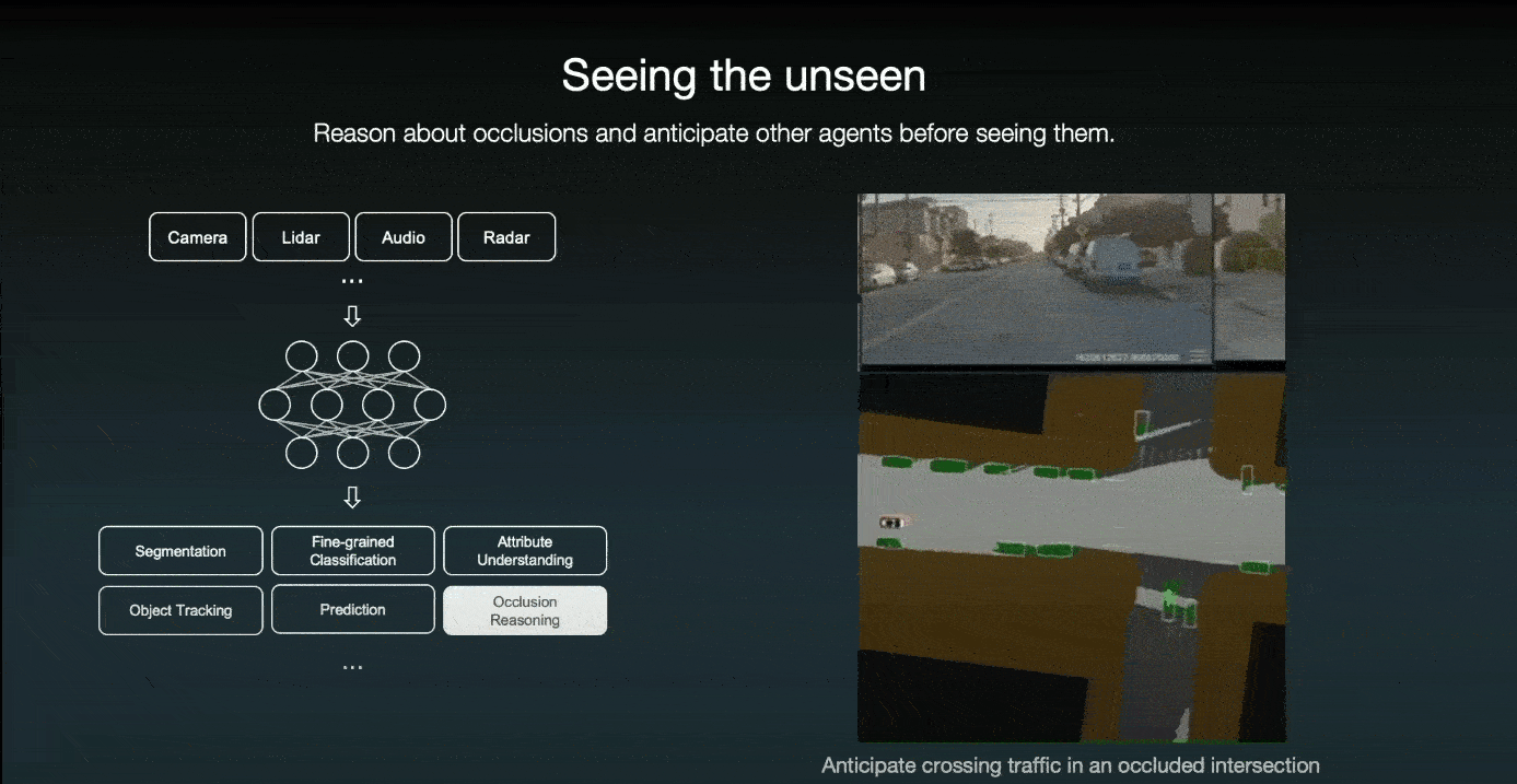
The other example is that prior to driving through an intersection, even if the system does not see any cross-traffic due to occlusion, the system imagines a car crossing from the right and slowing down; if it does see a car approaching, the autonomous car can stop in time.
Thus, regardless of what occurs in the future, the car will always be prepared to make prudent choices. All of this is due to the high-quality data that was used to train the model.
Additionally, they developed a few-shot active learned classifier for the purpose of mining-specific behaviors. For instance, if we want to train a model to predict when bikes will make a u-turn and want to find similar trajectories, a naive similarity search using embedding features would return left-turn scenarios. Because the two behaviors are somewhat similar and left-turning is a much more common occurrence than u-turning. However, with the assistance of human supervision, we can train a classifier with much fewer data and a higher degree of accuracy and return a variety of true positive u-turn examples.
Cruise also employs Reinforcement Learning (RL) to develop a safe policy. This application of RL was one of the aspects of the Cruise Under the Hood event that I enjoyed the most. Take the following example:
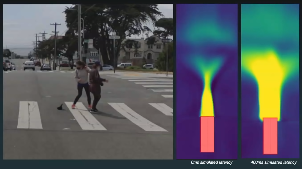
This scenario is possible on a regular basis, but we may not have it in the dataset. To deal with these situations, they use reinforcement learning to train an offline policy to understand what happens when pedestrians are extremely close to the ego car. They simulate decades of data in order to develop a cautious policy. As illustrated in the image, there are two representations of how a policy appears. Let us begin with the left one. If the pedestrian is in the yellow zone, they are in a very dangerous stage; they can run towards the vehicle or to the side, but if the vehicle is traveling at a high initial velocity, a collision is possible. Thus, the learned and safe policy would be to exercise caution if the pedestrian enters the yellow zone, as we have no idea what they will do.
Now, let us discuss the right one. They can train policy offline using a simulated latency, in this case 400 milliseconds, and as can be seen in the image, the yellow area is significantly larger and extends to the vehicle's sides. Because of the system's latency, we must exercise more cautiously.
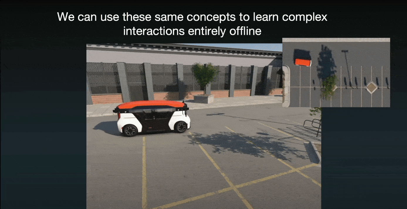
Additionally, they use simulation to learn policies offline for complex interactions involving multiple actors. For instance, the following video demonstrates two vehicles attempting to park. The same technique can be applied to the learning of a wide variety of behaviors both offline and in a simulator. Additionally, it can be used to generate data that they do not have or that is difficult to obtain.
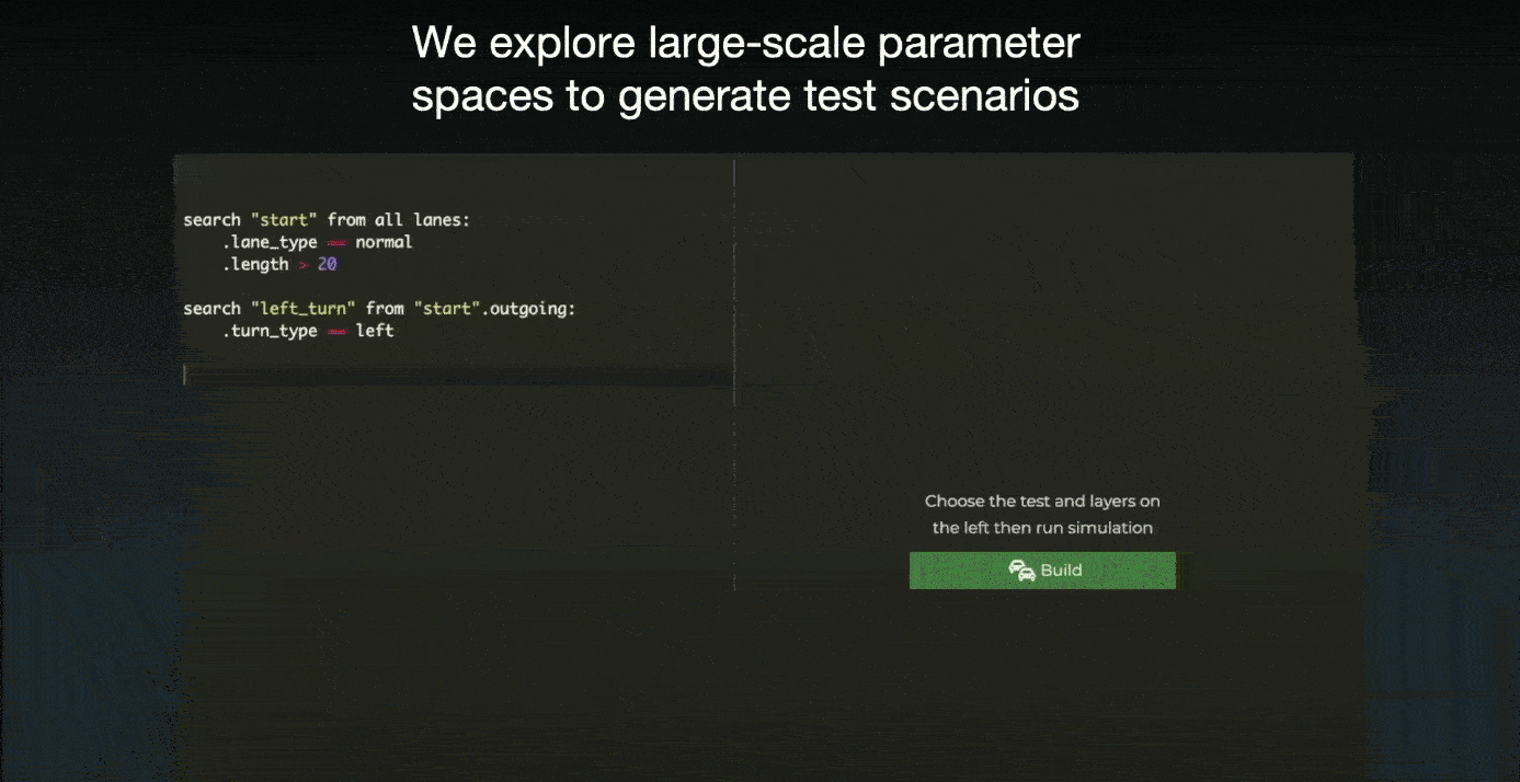
The other reason for using simulation in Cruise, which they refer to as Morpheus, is for safety. Simulation can be used to practice handling longtails and gradually reduce the reliance on real-world testing. Because longtails occur only once every thousands of road miles, testing the model in those scenarios will take a long time and is not scalable. Cruise has developed a system for exploring large-scale parameter spaces in order to generate test scenarios on a scalable basis. They can begin their simulation by searching for a specific location on the map. The following video demonstrates how they can generate a large and diverse test suit specific to a given situation. Beginning 15 meters before a left turn and then adding a straight road intersection with the turn and maybe adding an unlimited number of other parameters. It's astounding!
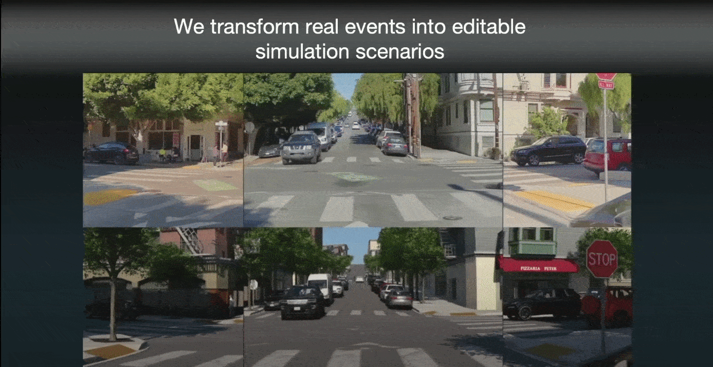
The next step is to introduce additional agents into the scene. They accomplish this through the process of converting real-world events into editable simulation scenarios dubbed road to sim. It combines perception data with heuristics developed over millions of real-world miles to recreate a complete simulation environment from road data. The following video depicts a simulation of a recreated scenario (bottom one) from the real world (top one). Then, while the scenario is running in simulation, we can experiment with various parameters and attributes.
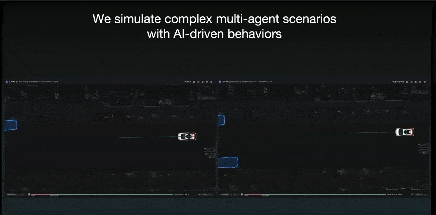
To increase the realism of the simulation, they use an artificial intelligence system called NPC (non-player character - a term borrowed from video games) AI to simulate the complex multi-agent behaviors of all agents in the scene except the autonomous car. The following are two variations on a single simulated environment in which an NPC is used to provide life to other agents:
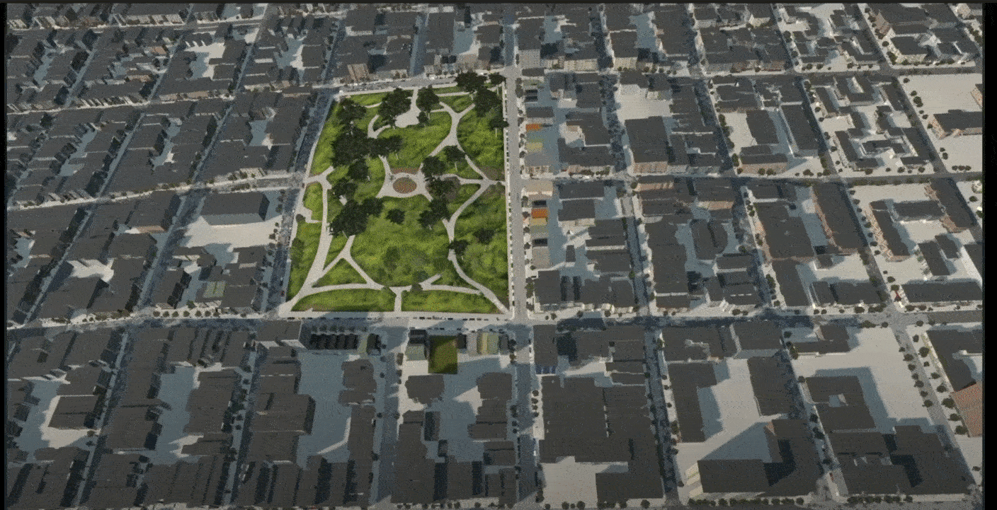
Along with the previously mentioned technologies, Cruise employs another called World-Gen to expand their business into new cities. It is capable of procedurally generating an entire city, with roads, curbs, sidewalks, lane markings, street lights, traffic signs, buildings, automobiles, and pedestrians. Here is the automatically generated Alamo Square Park in San Francisco:
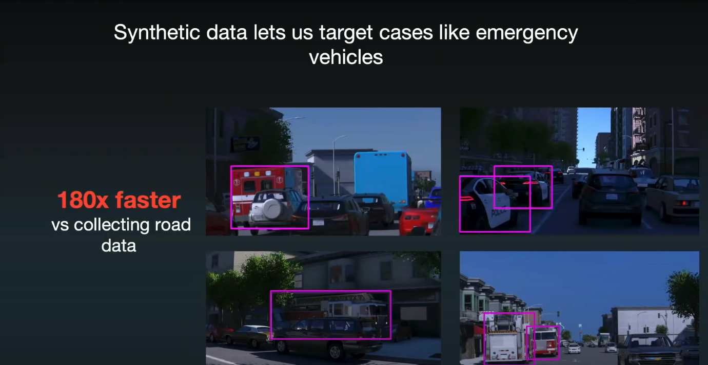
Additionally, they create high-quality simulations of various sensors and use them to generate synthetic data for the perception module and also collect data for instances such as emergency vehicles, which are uncommon and difficult to collect in the real world, and we need to detect them extremely precisely:
Furthermore, the simulation can be used to evaluate the algorithms' comfort and safety.
There is a lot of cool stuff they announced at the event. I highly encourage you to watch the event below:
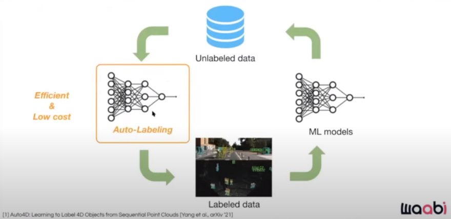
Waabi
In a recent workshop on self-supervised learning for autonomous driving at ICCV 2021, Raquel Urtasun talked about their labeling mechanisms at Waabi. She mentions that there is no need for humans in the labeling loop and it is possible to make the entire loop automatic.
Here is the Autonomy workflow used at Waabi:
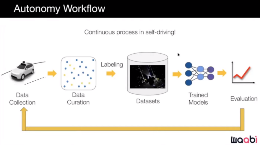
We have access to a fleet of vehicles as well as data collection platforms. So while we can collect a large amount of data, labeling it all is prohibitively expensive. Change and evolution of datasets, on the other hand, is necessary and occurs frequently in industry and the real world. However, because the world is changing as we drive to different cities, seeing different scenes and situations, and the city changing due to, for example, constructions, we need to change our datasets and train our models on them in order to be able to handle the situations that we see and cannot handle. Annotating these datasets is costly and the solution for that can be data curation.
In order to select samples in data to label, there are several techniques.
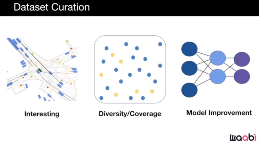
Interesting
We can choose a data point that we believe is interesting, exciting, and would be beneficial to learn about, whether for training or testing purposes.
They have some measures in place to select data from the logs and data collected by each of the vehicles. They accomplish this by using an intermediate process to tag logs with various properties, which they can then use to generate various notions of what might be interesting. They then rank and select the best examples. Automation is critical in this process.
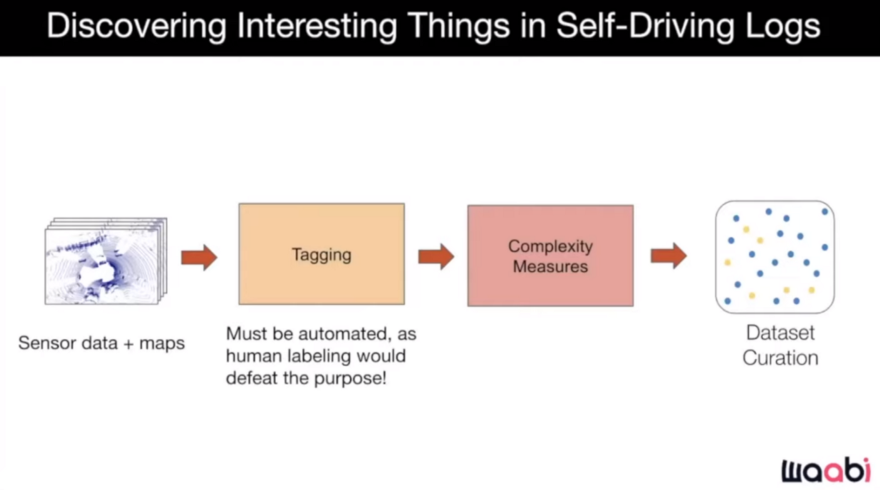
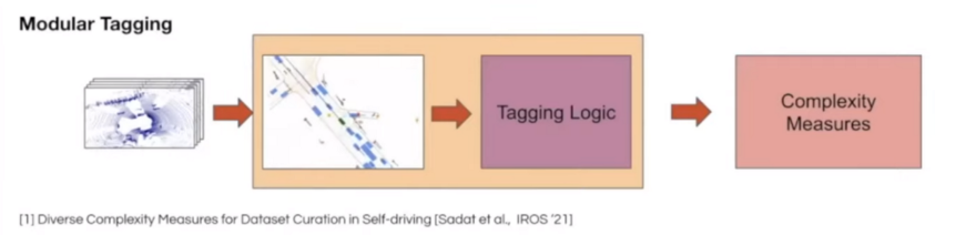
While humans are capable of tagging, the process must also be automated. They've devised two distinct methods for automatic tagging. The first is modular tagging, which involves running the perception system in offline mode on data to perform detection, tracking, prediction, and so on, and then determining whether the data is interesting and also determining the scene's complexity.
The other approach is to use a learning-based approach. Basically, you can learn to tag through the use of a sophisticated neural network. Then you can have sophisticated tags about what is happening in the scene and then use those for complexity measures.
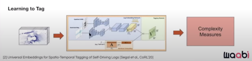
Here we focus on the modular tagging approach.
Each scenario, which is a few seconds of driving, has tags, HDMap, information about the self-driving car, and all other traffic participants. They then calculate complexity measures and combine them to arrive at a single value for the scene's complexity. Then, all of the scenarios will be ranked according to their complexity, and the top ones will be chosen.
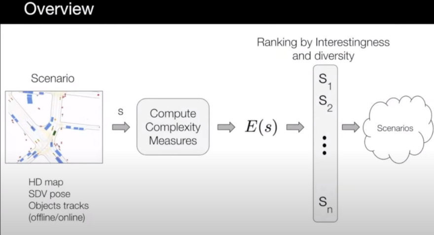
So, how can we say a scenario is complex and interesting for us to be selected? It can be many things: map complexity measures, actor complexity measures, and Self-Driving Vehicle (SDV) complexity measures.
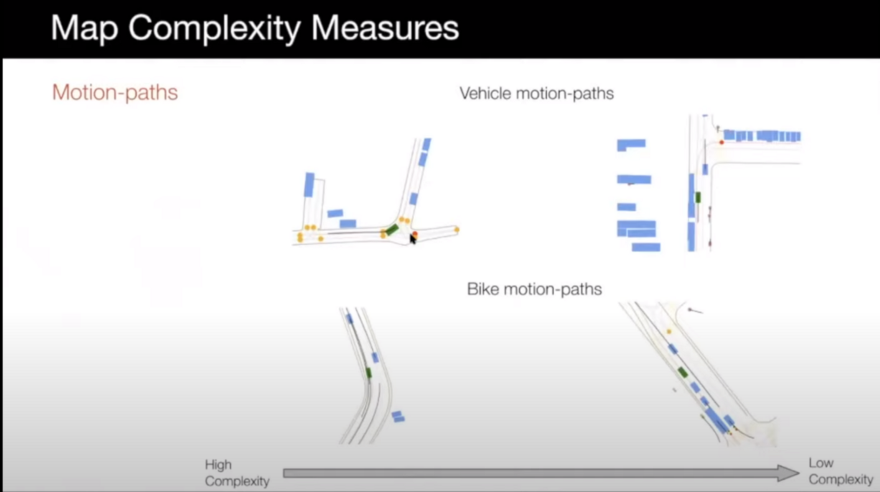
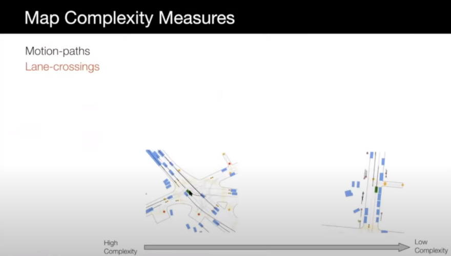
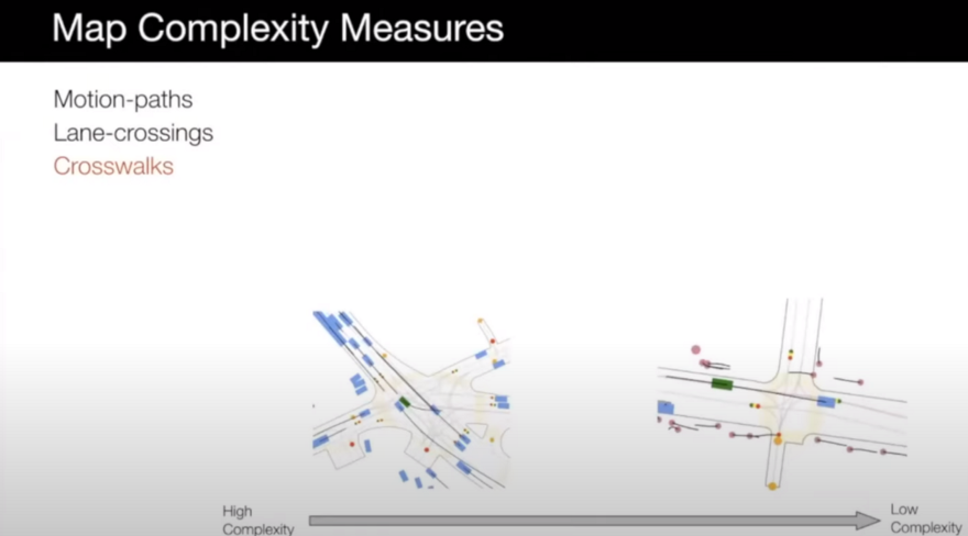
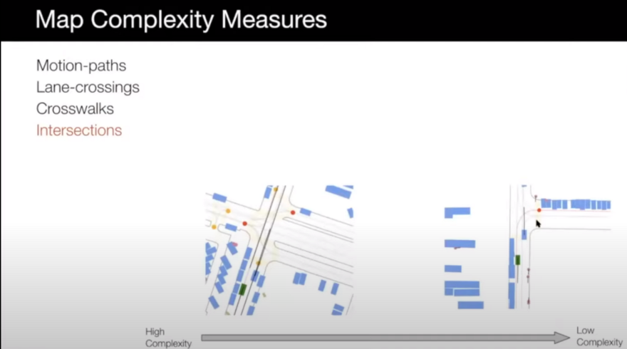
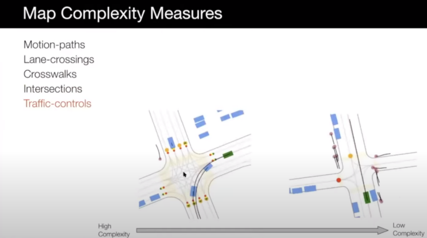
For the map complexity case, scenarios can be selected based on the following items ( In the following images, left is more complex and right is less complex):
- Motion paths: like high curvature roads or roads with odd shapes can be more interesting and have higher complexity.
- Lane-crossing: for example, an intersection where there are many lanes crossing each other and the car can go from different lanes to other lanes.
- Crosswalks: Scenarios with more crosswalks that might have more pedestrians can be more complex than others.
- Intersections: scenarios with more complex intersections can be interesting too. The left intersection has a more complex topology compared to the right one which is a very common and classic intersection.
- Traffic-controls: Intersections with many traffic lights that control many different things are more interesting.
- Map slope: scenarios with different slopes of the map and ground can be interesting and you need to make sure that your self-driving car can handle those too.
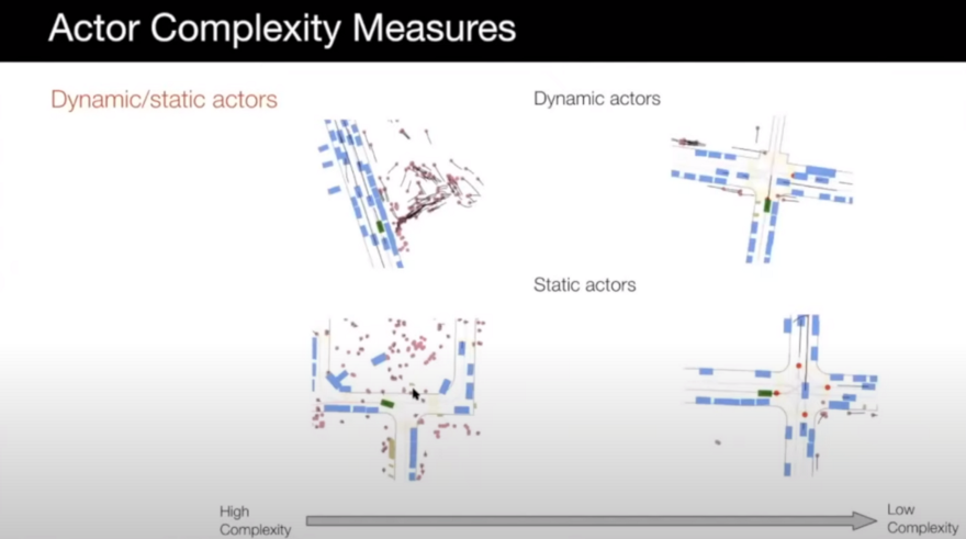
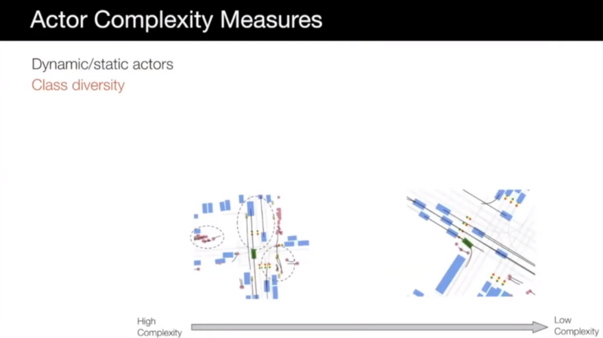
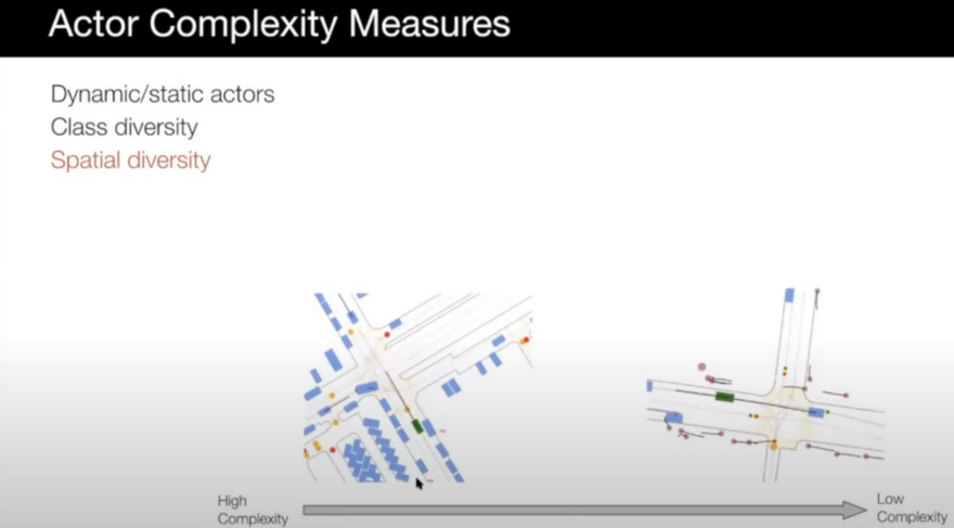
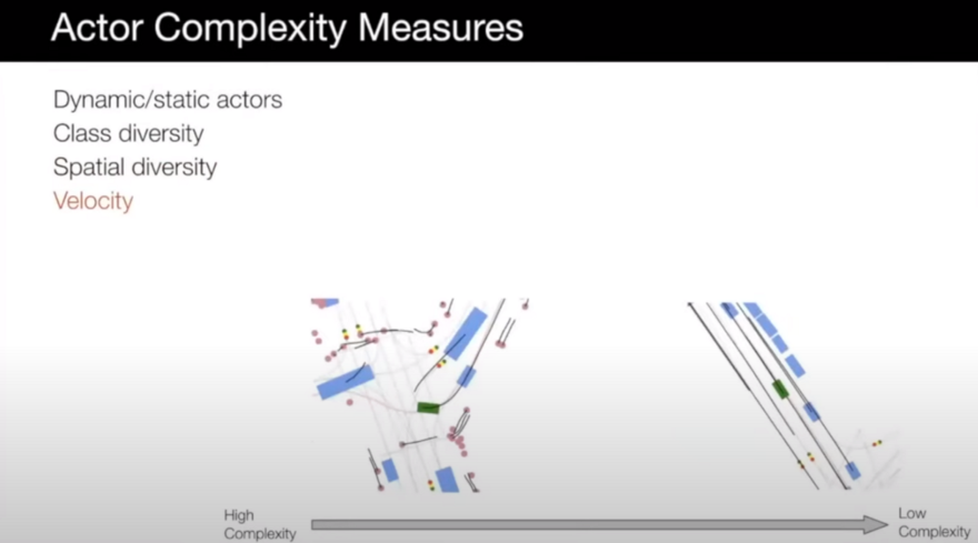
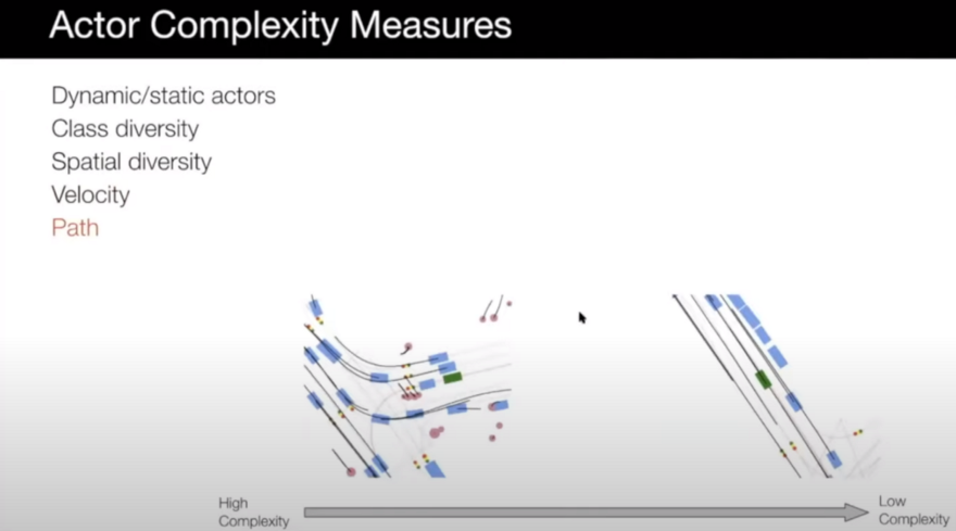
For actor complexity measures, the following cases can be considered:
- Dynamic or static actors: scenarios with more actors can be more complex and interesting and our self-driving car needs to be able to handle them.
- Class diversity: scenarios with various classes such as bicycles, pedestrians, animals, vehicles, etc., are more complex.
- Spatial diversity: scenarios that actors are in different locations in the scene can be interesting.
- Velocity: scenarios with actors with diverse velocities can be more complex.
- Path: variability of the path in the scenario can make it complex too.
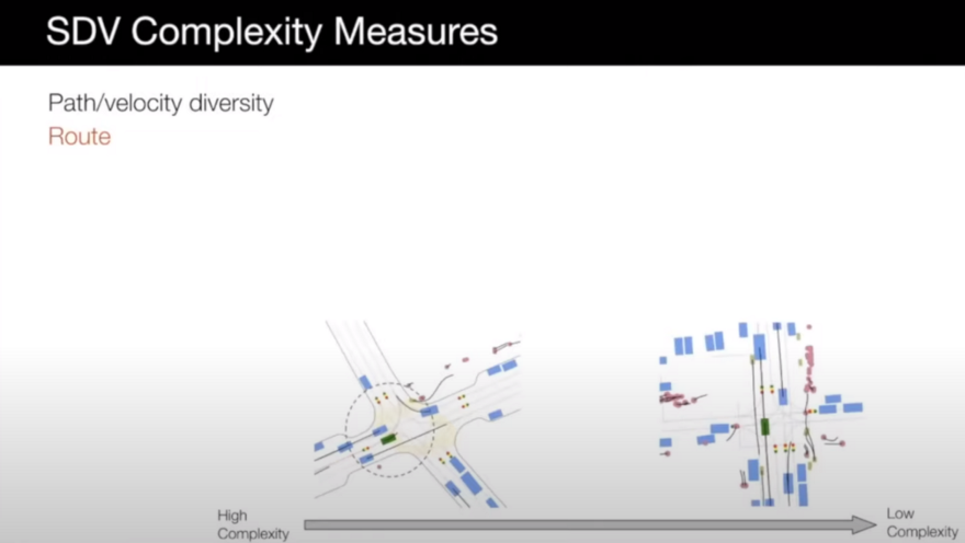
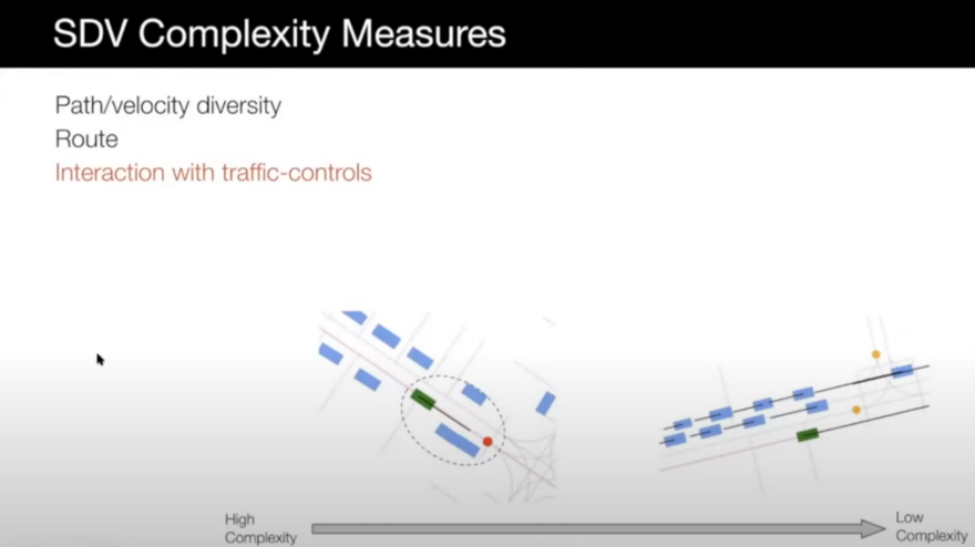
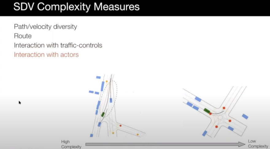
The other case that can be considered for complexity measurement is the SDV complexity measure. The following items can be important in this case:
-
Path/Velocity diversity: it is similar to the previous two items in the actor complexity measures case.
-
Route: route of the SDV can make a scenario more complex. For example, in an intersection, turning is more complex than going straight.
- Interaction with traffic lights: scenarios that the SDV needs to deal with traffic lights can be more complex.
- Interaction with actors: we can also look at how do we interact with other actors. Is somebody cutting in front of us? Is somebody slowing down behind us? Is somebody entering our line? These are pretty interesting scenarios that we need to make sure our car can handle.
For more details on the mentioned measures, check the paper "Diverse Complexity Measures for Dataset Curation in Self-driving".
After selecting interesting and complex scenarios based on the mentioned measures, we can label them. What is important to note is that depending on what is your goal and what are you interested in, for example, object detection or motion forecasting, or motion planning, certain things would be more interesting than others. The way to handle this would be very simple. We can compute the weighted sum of these complexity measures in order to project this high-dimensional vector into a single number.
In summary, the complexity of each scenario based on each one of the above-mentioned items will be calculated, and based on the task, the weight vector will be selected and multiplied by these complexity measures to calculate a single number for that scenario.
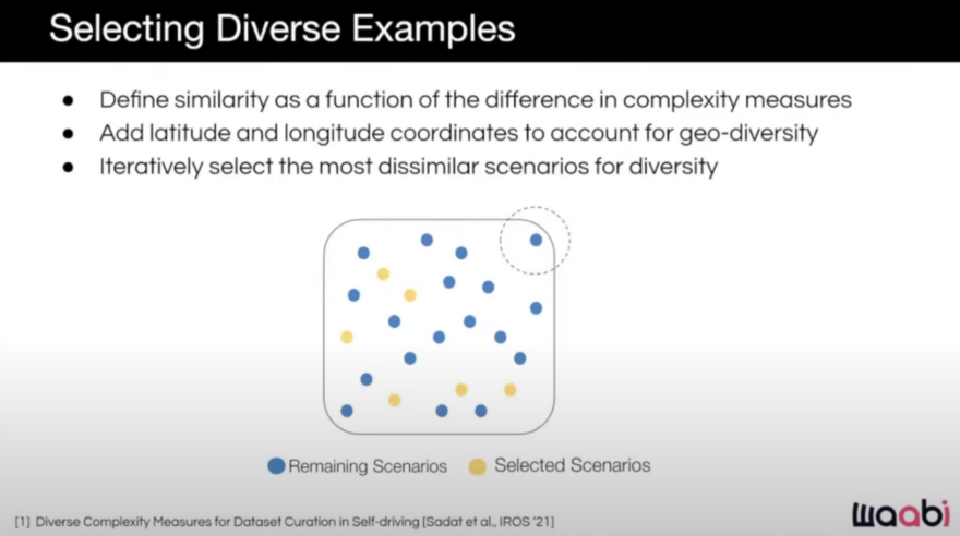
Diversity/Coverage
In addition to the scenarios that are interesting, we should consider the dataset's diversity and coverage. At the end of the day, we are attempting to develop vehicles capable of operating within our operational domain, and we must ensure that they are trained to handle all possible situations.
One way to handle this is that as soon as you have decided which scenarios you want to label so far, you can look at what do they miss. What are areas in your space that your current selected scenarios do not cover and the new scenario is far from them? It is also important to add geographical diversity here. Then, we can iteratively select examples that are far away from our selected scenarios and label them. We repeat this procedure until the selected dataset has enough diversity and there is no new data point far enough from the selected points.
Model Improvement
The other factor for selecting scenarios is model improvement. We can select data points that aid the model's performance improvement. So, the scenarios will be selected based on their expected improvement in the model performance or how much the model is uncertain about that scenario. Human intervention on the road can also be a notion of model failure in that scenario and shows that the scenario can be used to learn something from it. Basically, the active learning techniques that we mentioned at the beginning f this post can be used here.
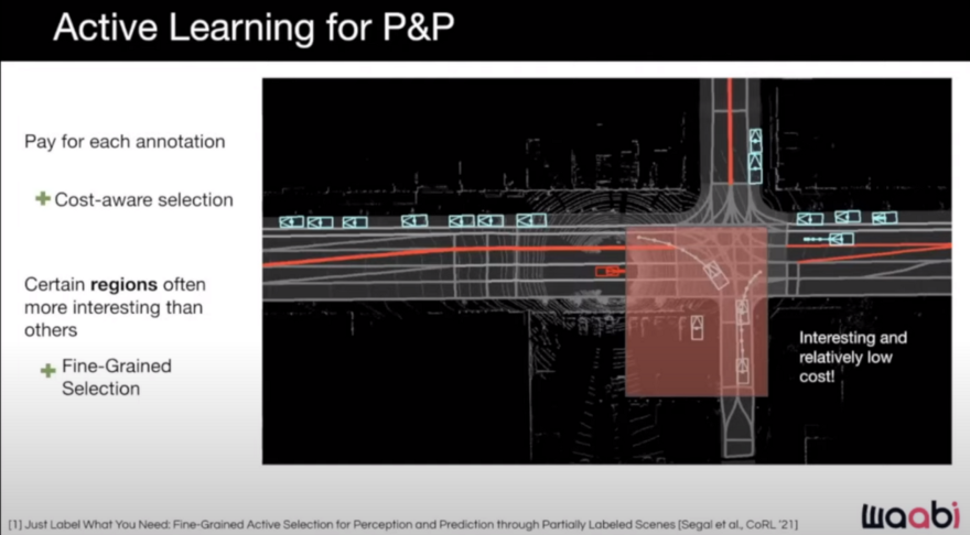
One point that needs to be taken into account is that, in addition to prioritizing some scenarios over others, we can think of more important regions in a scene. Some regions are more important than others and as we pay annotators per each click, it is important to select and label parts of the scene that are informative and reach and not all the scene. For example, in the following scene, the cars in the middle of the image are more important than the parked cars on the left road.
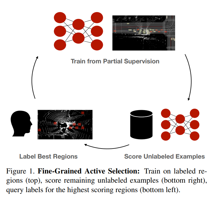
Here is the flowchart they propose in their paper called "Just Label What You Need: Fine-Grained Active Selection for Perception and Prediction through Partially Labeled Scenes":
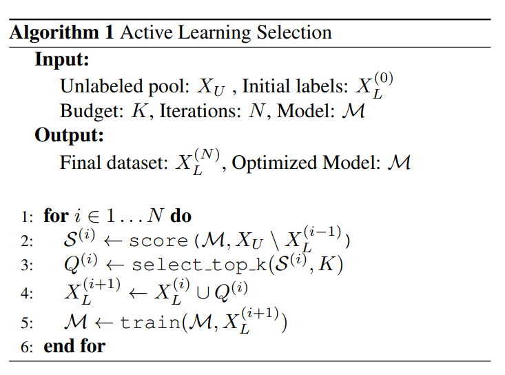
Scoring the unlabeled examples can be based on the mentioned scores such as Entropy. And here is their proposed algorithm:
After selecting scenarios based on their interestingness, diversity/coverage, and model improvement we need to label them.
The good news is that we don't need to do this auto-labeling in online mode. So we can use more sophisticated models in offline mode without worrying about latency and other online inference bottlenecks. We also have access to past and future timesteps which can help in the annotation.
For example, for the task of labeling a trajectory of an object with its bounding boxes, first, we can run the offline model to give us the first estimate of where are all actors in the scene as well as how they are moving, and then we are going to have sophisticated ways of correcting these results to have better trajectories. Here is the method they propose in the paper called "Auto4D: Learning to Label 4D Objects from Sequential Point Clouds":
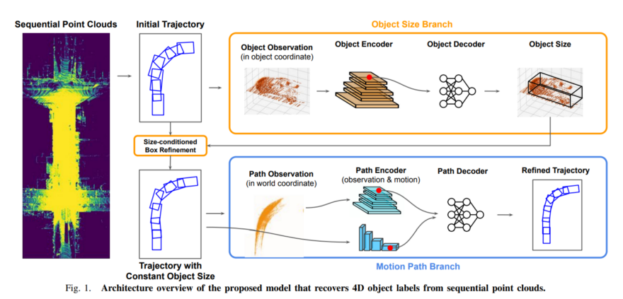
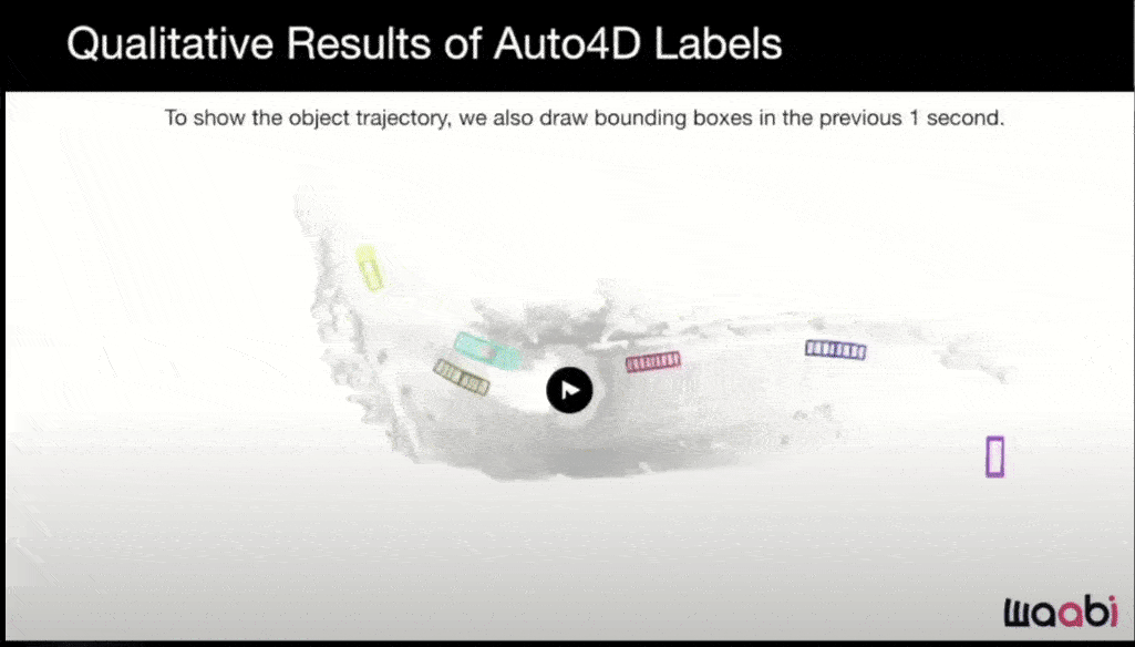
There are two branches in this approach. The first is to get the initially estimated trajectory and fix the size of the object. Then the second branch gets the trajectory with fixed size and also the point cloud of the object across time frames and fuses them and outputs a refined trajectory. Here is the result with very nice and smooth trajectories:
As with previous companies we've reviewed, Waabi makes extensive use of simulation.
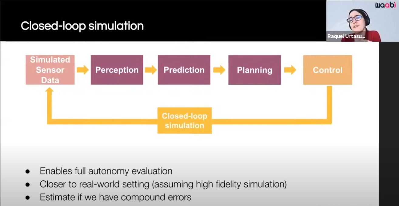
Training is conducted using a 3D, real-world, high-fidelity simulation, which enables training on uncommon scenarios and eliminates the need for field data collection. In other words, there is no reason to drive "millions of miles" and create potentially dangerous situations or even collisions.
Furthermore, having a fleet of hundreds of vehicles on the road is prohibitively expensive, and it can be dangerous. Rather than that, Waabi employs an AI approach that is capable of learning from fewer examples and scaling.
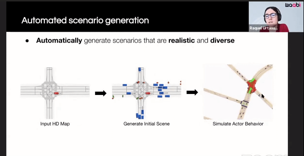
Rather than requiring humans to design 3D assets by hand and engineers to implement rule-based simulation behavior, Waabi generates virtual worlds and multi-agent systems automatically based on observed human driving behavior.
Here are the components of their closed-loop simulation system:
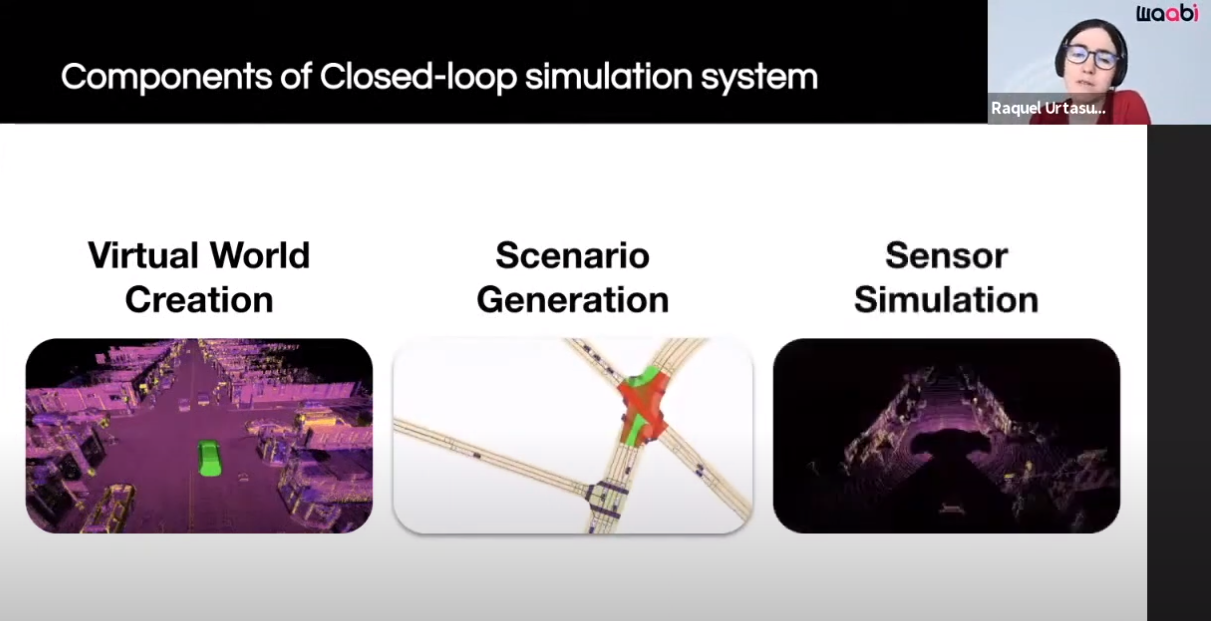
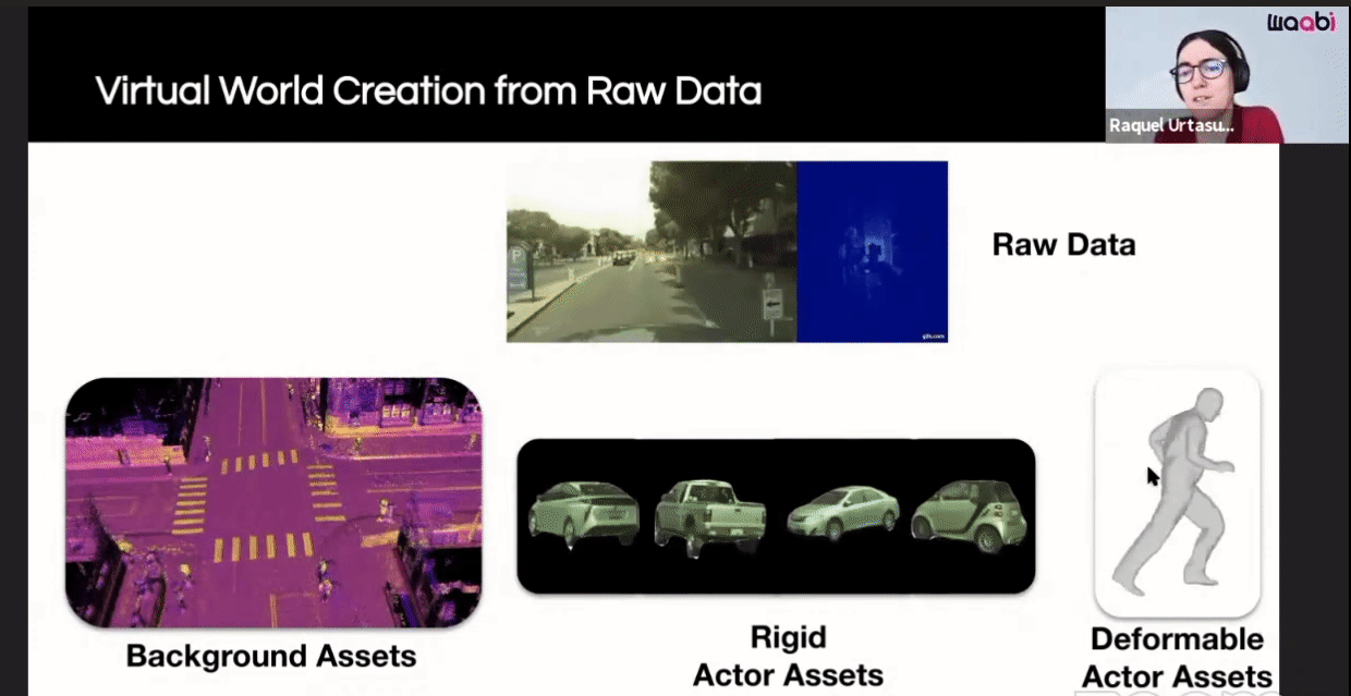
The first component is the Virtual World Creation. Generating the background, cars, pedestrians and animating them are done in this component.
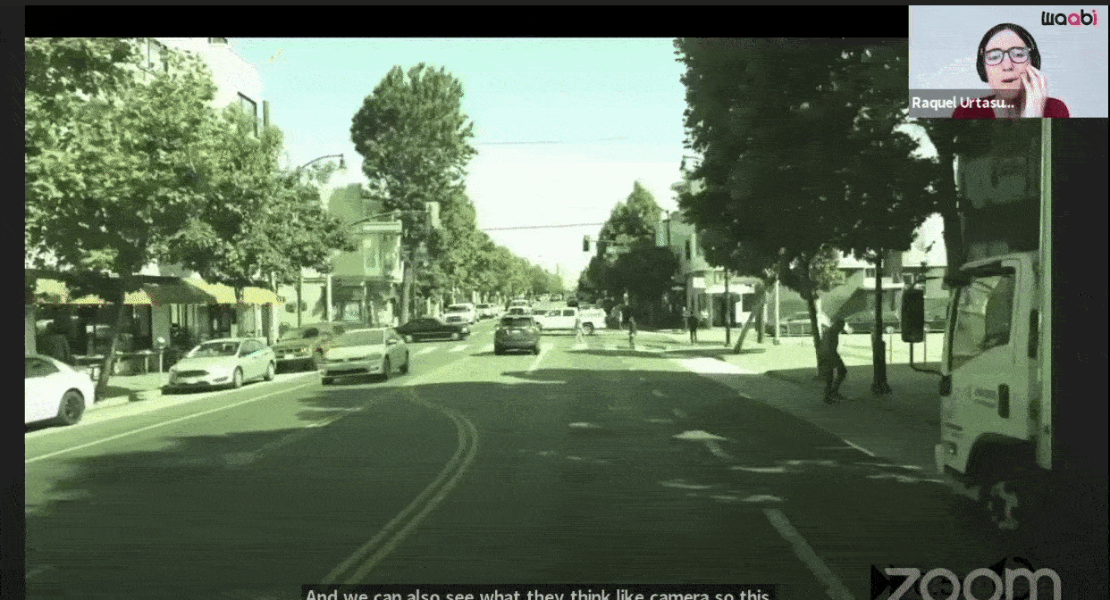
Additionally, Waabi models sensor noise using AI and physics, resulting in perception outputs that behave similarly in both simulation and the real world. The following videos show the simulated LiDAR and Camera sensor data in comparison to real data:
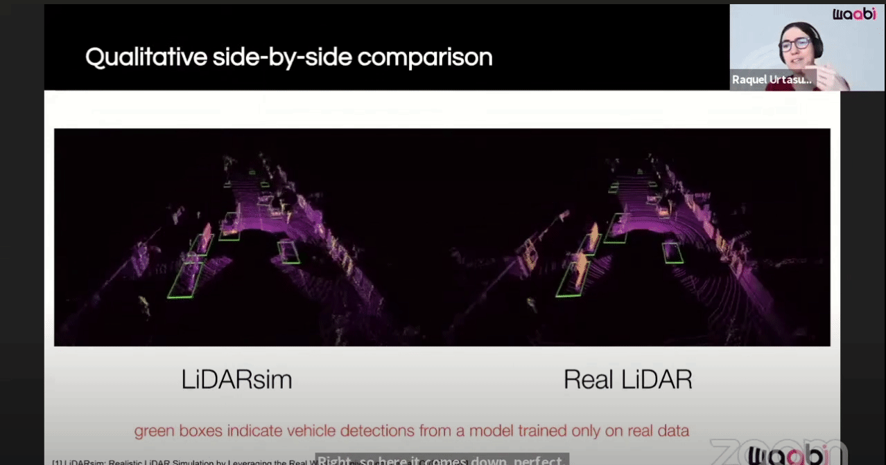
Some objects in the above video are fake and generated to make the scene more complex!
If you want to know more details about their LiDAR simulation, check their LiDARsim paper.
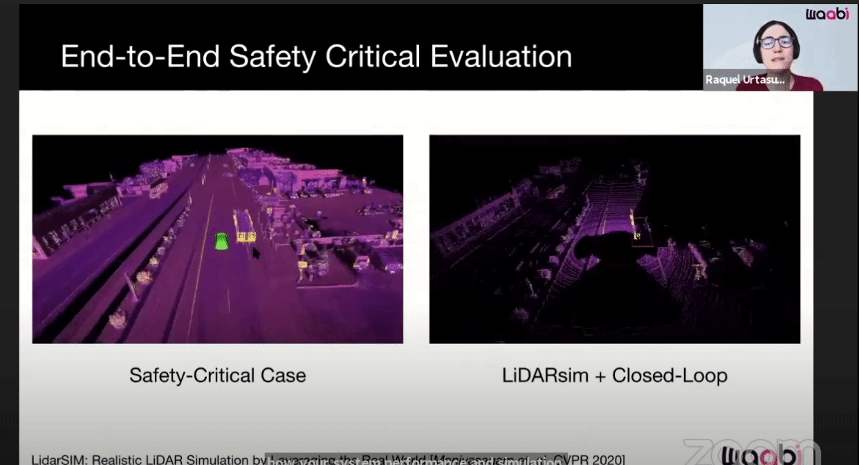
Then they use the simulator to test simple scenarios or those that occur frequently, as well as those that occur infrequently. Also, they can create safety critical cases and test their models there.
That's it for Waabi! Let's go for the last company.
Aurora
Aurora, on the other hand, takes a slightly different approach. Rather than blindly pushing for increased mileage, they've maintained a focus on collecting high-quality real-world data and extracting the maximum value from each data point. For instance, they amplify the impact of real-world experience by identifying interesting or novel events and incorporating them into their Virtual Testing Suite, where they are used to continuously improve the Aurora driver.
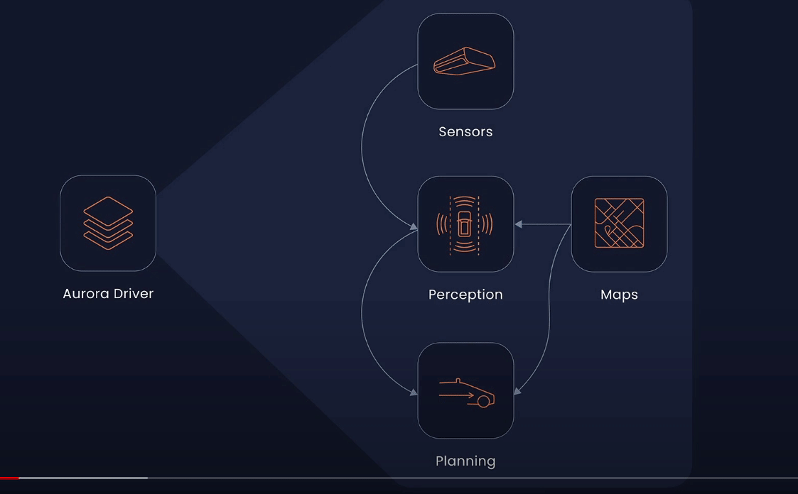
Aurora DriverHowever, not all real-world events are amenable to simulation in virtual environments. For instance, the exhaust of a vehicle may be of interest to an object detection system. Thus, using real-world data from such scenes to train the perception system to recognize and ignore exhaust can result in a more enjoyable driving experience.
The on-road events that they turn into virtual tests come from two sources:
-
Copilot annotations: Vehicle operator copilots, who provide support from the passenger's seat, routinely flag experiences that are interesting, uncommon, or novel. They frequently recreate these in their Virtual Testing Suite to familiarize the Aurora Driver with a variety of road conditions.
-
Disengagements: when their vehicle operators proactively retook control when they suspected an unsafe situation was about to occur or when they disliked the way the vehicle was driving.
Their Virtual Testing Suite is a complementary collection of tests that evaluate the software's functionality at every level. As a result, they transform real-world events into one or more of the following virtual tests (read more here):
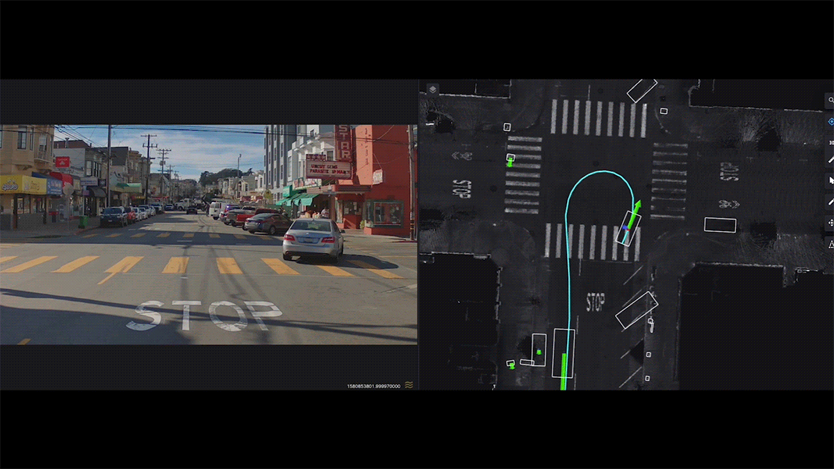
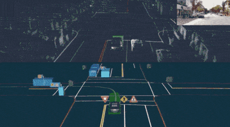
- Perception tests: Consider the following scenario: a bicyclist passes one of their vehicles. Specialists review the event's log footage and then label items such as the object category (bicyclist), the velocity (3 mph), and so on. They can then use this "absolute truth" to assess the ability of new versions of perception software to accurately determine what occurred on the road. Here is an example of the labeling procedure:
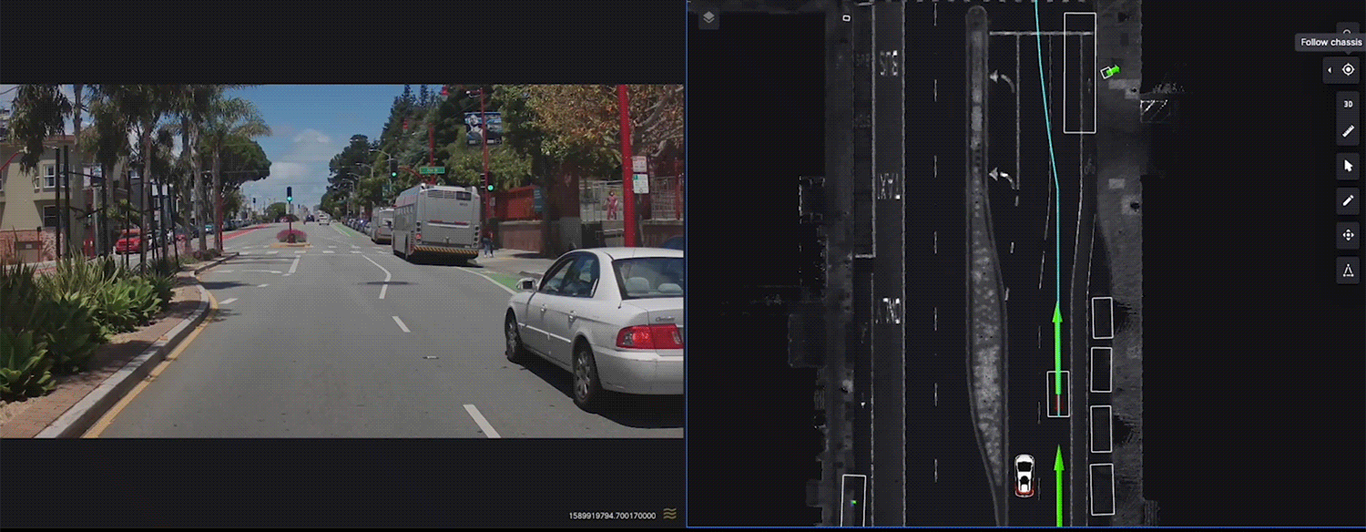
- Manual driving evaluations: They compare the planned trajectory of the Aurora Driver to the actual trajectory of the vehicle operator and test whether their motion planning software can accurately forecast what a trained, expert driver would do in complex situations: (comparing a vehicle operator's trajectory (blue) to the intended trajectory of the Aurora Driver (green) during a right turn).
- Simulations: Simulations are virtual representations of the real world in which the Aurora Driver can be tested in numerous permutations of the same situation. Additionally, simulations enable them to simulate a wide variety of interactions between the Aurora Driver and other virtual world actors. For instance, how will a jaywalker react when the Aurora Driver comes to a halt? And then, how do the simulation's other actors react when the jaywalker crosses the street?
By utilizing their online-to-offline pipeline, they convert on-road events into virtual tests:
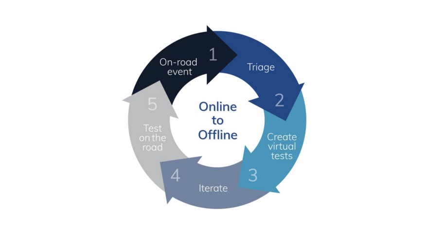
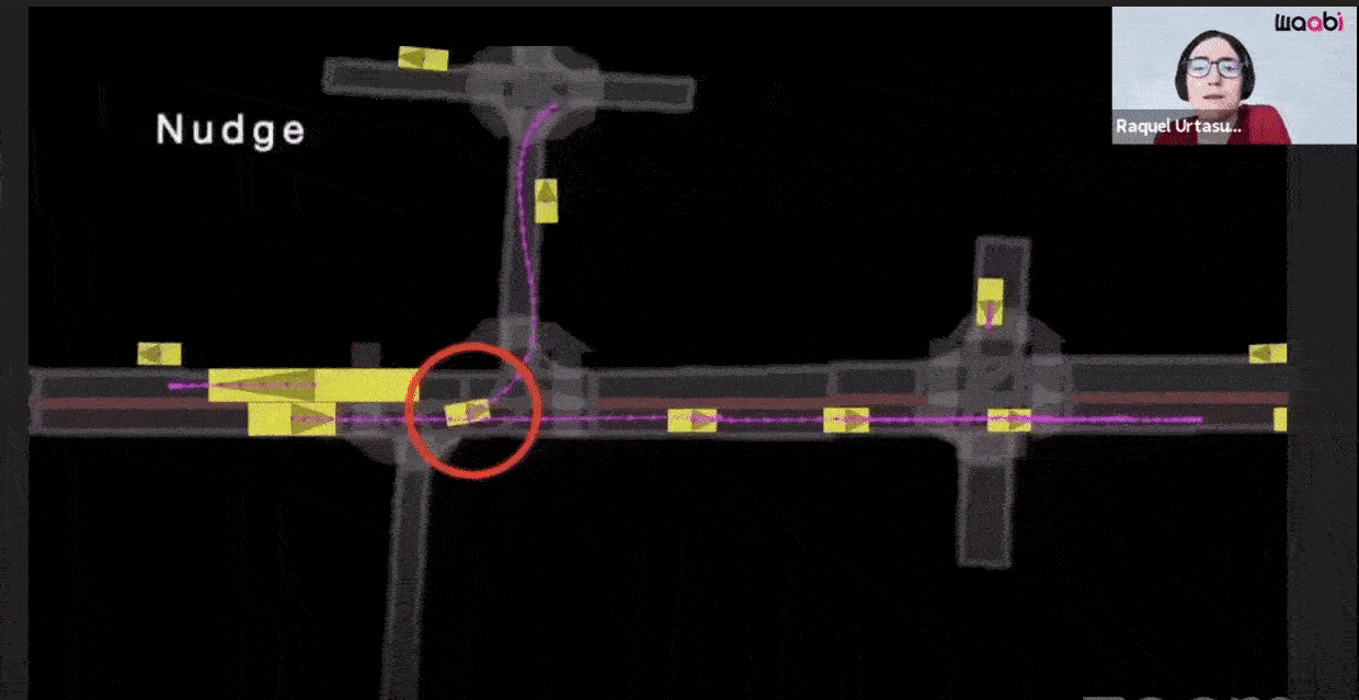
Let's review this process by an example of a disengagement that helped the Aurora Driver learn how to nudge (when the Aurora Driver adjusts its trajectory to move around obstacles).
-
On-Road Event: Vehicle operators annotate disengagements and highlight scenes that are unusual, novel, or interesting. The Aurora Driver hesitates in this situation to nudge around a vehicle that abruptly veers off the roadway and into an on-street parking space. To avoid causing traffic disruptions, the trained vehicle operators quickly take control and drive around the parked vehicle.
-
Triage: The triage team conducts an examination of on-road incidents and provides an initial diagnosis. For instance, AV must nudge a vehicle to pull over and come to a complete stop. #motionplanning
-
Create virtual tests: They develop one or more simulated tests, which may include perception tests, manual driving evaluations, and/or simulations. They used it as the basis for 50 new nudging simulations, which included a recreation of the exact scene from the disengagement log footage and variations created by altering variables such as the speed of the vehicle in front of the ego car.
-
Iterate: The diverse Virtual Testing Suite enables engineers to fine-tune new and existing capabilities. The engineering team fine-tuned the Aurora Driver's ability to nudge using the nudging simulations inspired by this disengagement, as well as numerous other codebase tests (unit and regression), perception tests, and manual driving evaluations.
-
Test on the road: They put enhancements to the test in the real world and continue to collect useful data. Here is the Aurora Driver nudging gracefully through a complex situation: