Data Engineering - Week 3

• Data Warehouse
  • OLTP vs OLAP
  • Data Warehouse
  • BigQuery
    • Partitioning
    • Clustering
    • Direct Import (Managed Tables)
    • Query without Loading (External Tables)
    • Machine Learning in BigQuery
  • Amazon Redshift
    • Machine Learning in Redshift
• Conclusion

Note: The content of this post is from the course videos, my understandings and searches, and reference documentations.

Data Warehouse

OLTP vs OLAP

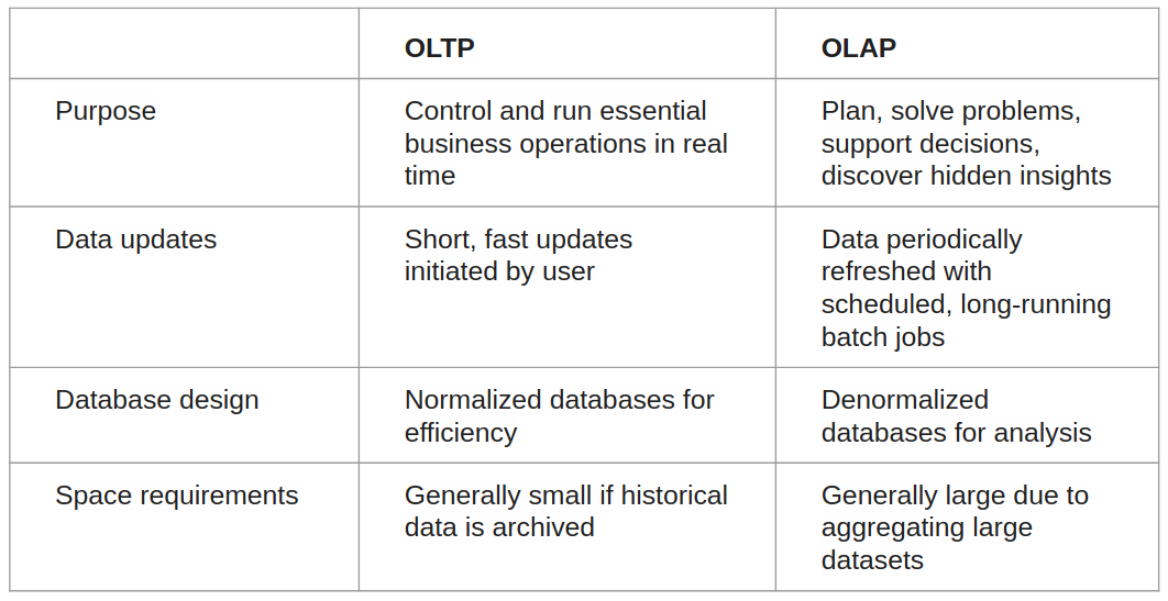
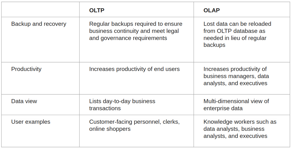
The two terms look similar but refer to different kinds of systems. Online transaction processing (OLTP) captures, stores, and processes data from transactions in real time. Online analytical processing (OLAP) uses complex queries to analyze aggregated historical data from OLTP systems.

An OLTP system is a database that captures and retains transaction data. Individual database entries made up of numerous fields or columns are involved in each transaction. Banking and credit card transactions, as well as retail checkout scanning, are examples. Because OLTP databases are read, written, and updated frequently, the emphasis in OLTP is on fast processing. Built-in system logic protects data integrity if a transaction fails.

For data mining, analytics, and business intelligence initiatives, OLAP applies complicated queries to massive amounts of historical data aggregated from OLTP databases and other sources. The emphasis in OLAP is on query response speed for these complicated queries. Each query has one or more columns of data derived from a large number of rows. Financial performance year over year or marketing lead generation trends are two examples. Analysts and decision-makers can utilize custom reporting tools to turn data into information using OLAP databases and data warehouses. OLAP query failure does not affect or delay client transaction processing, but it can affect or delay the accuracy of business intelligence insights. [ref]

Data Warehouse

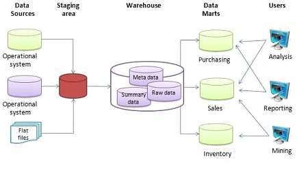
A data warehouse (DW or DWH), often known as an enterprise data warehouse (EDW), is a reporting and data analysis system that is considered a key component of business intelligence. DWs are central data repositories that combine data from a variety of sources. They keep current and historical data in one place and utilize it to generate analytical reports for employees across the company.

The data in the warehouse comes from the operating systems and is uploaded there (such as marketing or sales). Before being used in the DW for reporting, the data may transit via an operational data store and require data cleansing for extra procedures to ensure data quality.

The two major methodologies used to design a data warehouse system are extract, transform, load (ETL) and extract, load, transform (ELT). [wikipedia]

Google BigQuery, Amazon Redshift, and Microsoft Azure Synapse Analytics are three data warehouse services. Here we review BigQuery and Redshift.

BigQuery

BigQuery is a fully managed enterprise data warehouse that helps you manage and analyze your data with built-in features like machine learning, geospatial analysis, and business intelligence. BigQuery's serverless architecture lets you use SQL queries to answer your organization's biggest questions with zero infrastructure management. BigQuery's scalable, distributed analysis engine lets you query terabytes in seconds and petabytes in minutes.

BigQuery maximizes flexibility by separating the compute engine that analyzes your data from your storage choices. You can store and analyze your data within BigQuery or use BigQuery to assess your data where it lives. Federated queries let you read data from external sources while streaming supports continuous data updates. Powerful tools like BigQuery ML and BI Engine let you analyze and understand that data.

BigQuery interfaces include Google Cloud Console interface and the BigQuery command-line tool. Developers and data scientists can use client libraries with familiar programming including Python, Java, JavaScript, and Go, as well as BigQuery's REST API and RPC API to transform and manage data. ODBC and JDBC drivers provide interaction with existing applications including third-party tools and utilities.

As a data analyst, data engineer, data warehouse administrator, or data scientist, the BigQuery ML documentation helps you discover, implement, and manage data tools to inform critical business decisions. [BigQuery docs]

Partitioning

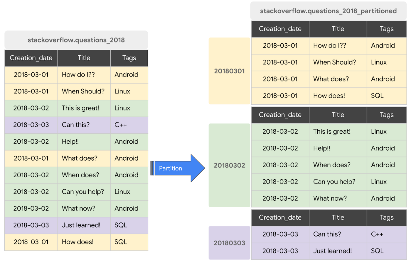
A partitioned table is a special table that is divided into segments, called partitions, that make it easier to manage and query your data. You can typically split large tables into many smaller partitions using data ingestion time or TIMESTAMP/DATE column or an INTEGER column. BigQuery’s decoupled storage and compute architecture leverages column-based partitioning simply to minimize the amount of data that slot workers read from disk. Once slot workers read their data from disk, BigQuery can automatically determine more optimal data sharding and quickly repartition data using BigQuery’s in-memory shuffle service. [source]

source

Check the previous video and also here to see an example of the performance gain.

The example SQL query can be like this:

CREATE OR REPLACE TABLE `stackoverflow.questions_2018_partitioned`
PARTITION BY
 DATE(creation_date) AS
SELECT
 *
FROM
 `bigquery-public-data.stackoverflow.posts_questions`
WHERE
 creation_date BETWEEN '2018-01-01' AND '2018-07-01';

Clustering

When a table is clustered in BigQuery, the table data is automatically organized based on the contents of one or more columns in the table’s schema. The columns you specify are used to collocate related data. Usually high cardinality and non-temporal columns are preferred for clustering.

When data is written to a clustered table, BigQuery sorts the data using the values in the clustering columns. These values are used to organize the data into multiple blocks in BigQuery storage. The order of clustered columns determines the sort order of the data. When new data is added to a table or a specific partition, BigQuery performs automatic re-clustering in the background to restore the sort property of the table or partition. Auto re-clustering is completely free and autonomous for the users. [source]

source

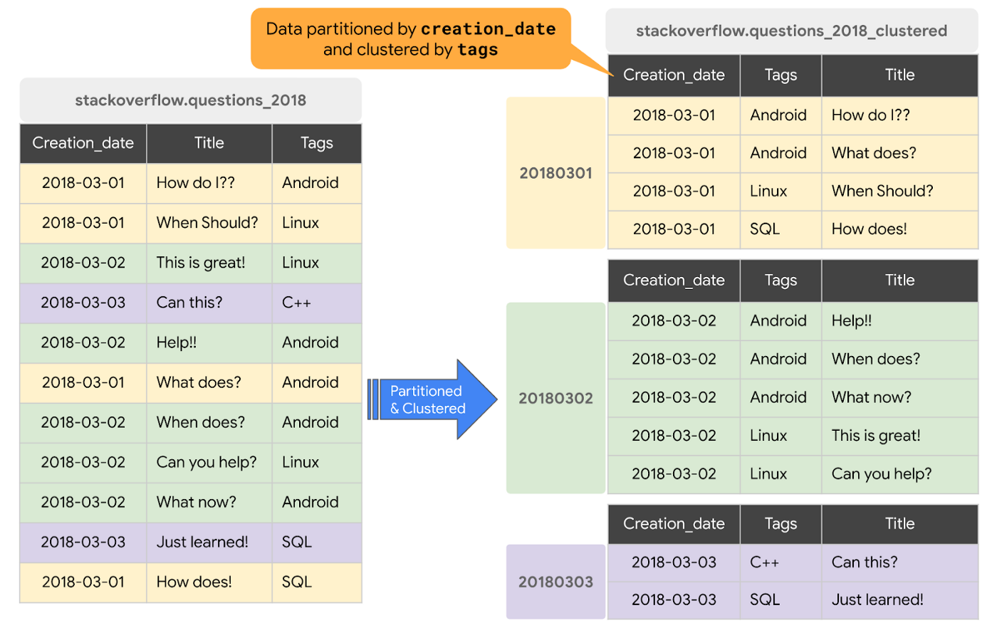
Clustering can improve the performance of certain types of queries, such as those using filter clauses and queries aggregating data. When a query containing a filter clause filters data based on the clustering columns, BigQuery uses the sorted blocks to eliminate scans of unnecessary data. When a query aggregates data based on the values in the clustering columns, performance is improved because the sorted blocks collocate rows with similar values. BigQuery supports clustering over both partitioned and non-partitioned tables. When you use clustering and partitioning together, your data can be partitioned by a DATE or TIMESTAMP column and then clustered on a different set of columns (up to four columns). [source]

Clustered tables in BigQuery are subject to the following limitations:

• Only standard SQL is supported for querying clustered tables and for writing query results to clustered tables.

• Clustering columns must be top-level, non-repeated columns of one of the following types:

• DATE

• BOOL
• GEOGRAPHY
• INT64
• NUMERIC
• BIGNUMERIC
• STRING
• TIMESTAMP

• DATETIME

• You can specify up to four clustering columns.

• When using STRING type columns for clustering, BigQuery uses only the first 1,024 characters to cluster the data. The values in the columns can themselves be longer than 1,024.

Check the previous video and also here to see an example of the performance gain.

The example SQL query can be like this:

CREATE OR REPLACE TABLE `stackoverflow.questions_2018_clustered`
PARTITION BY
 DATE(creation_date)
CLUSTER BY
 tags AS
SELECT
 *
FROM
 `bigquery-public-data.stackoverflow.posts_questions`
WHERE
 creation_date BETWEEN '2018-01-01' AND '2018-07-01';

Check the following video to learn more:

You can also chech this codelab to learn more about partitioning and clustering.

Let's now compare clustering and partitioning:

source

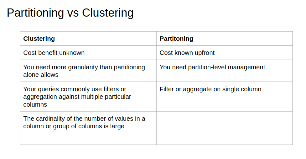
Now, let's see when we have to choose clustering over partitioning [ref]:

• Partitioning results in a small amount of data per partition (approximately less than 1 GB)
• Partitioning results in a large number of partitions beyond the limits on partitioned tables
• Partitioning results in your mutation operations modifying the majority of partitions in the table frequently (for example, every few minutes)

In order to have better performance with lower cost, the following best practices in BQ are useful:

• Cost reduction

  • Avoid SELECT *
  • Price your queries before running them
  • Use clustered or partitioned tables
  • Use streaming inserts with caution
  • Materialize query results in stages

• Query performance

  • Filter on partitioned columns
  • Denormalizing data
  • Use nested or repeated columns
  • Use external data sources appropriately
    • Don't use it, in case u want a high query performance
  • Reduce data before using a JOIN
  • Do not treat WITH clauses as prepared statements
  • Avoid oversharding tables
  • Avoid JavaScript user-defined functions
  • Use approximate aggregation functions (HyperLogLog++)
  • Order Last, for query operations to maximize performance
  • Optimize your join patterns
    • As a best practice, place the table with the largest number of rows first, followed by the table with the fewest rows, and then place the remaining tables by decreasing size.

Now let's see how to load or ingest data into BigQuery and analyze them.

Direct Import (Managed Tables)

BigQuery can ingest datasets from a variety of different formats directly into its native storage. BigQuery native storage is fully managed by Google—this includes replication, backups, scaling out size, and much more.

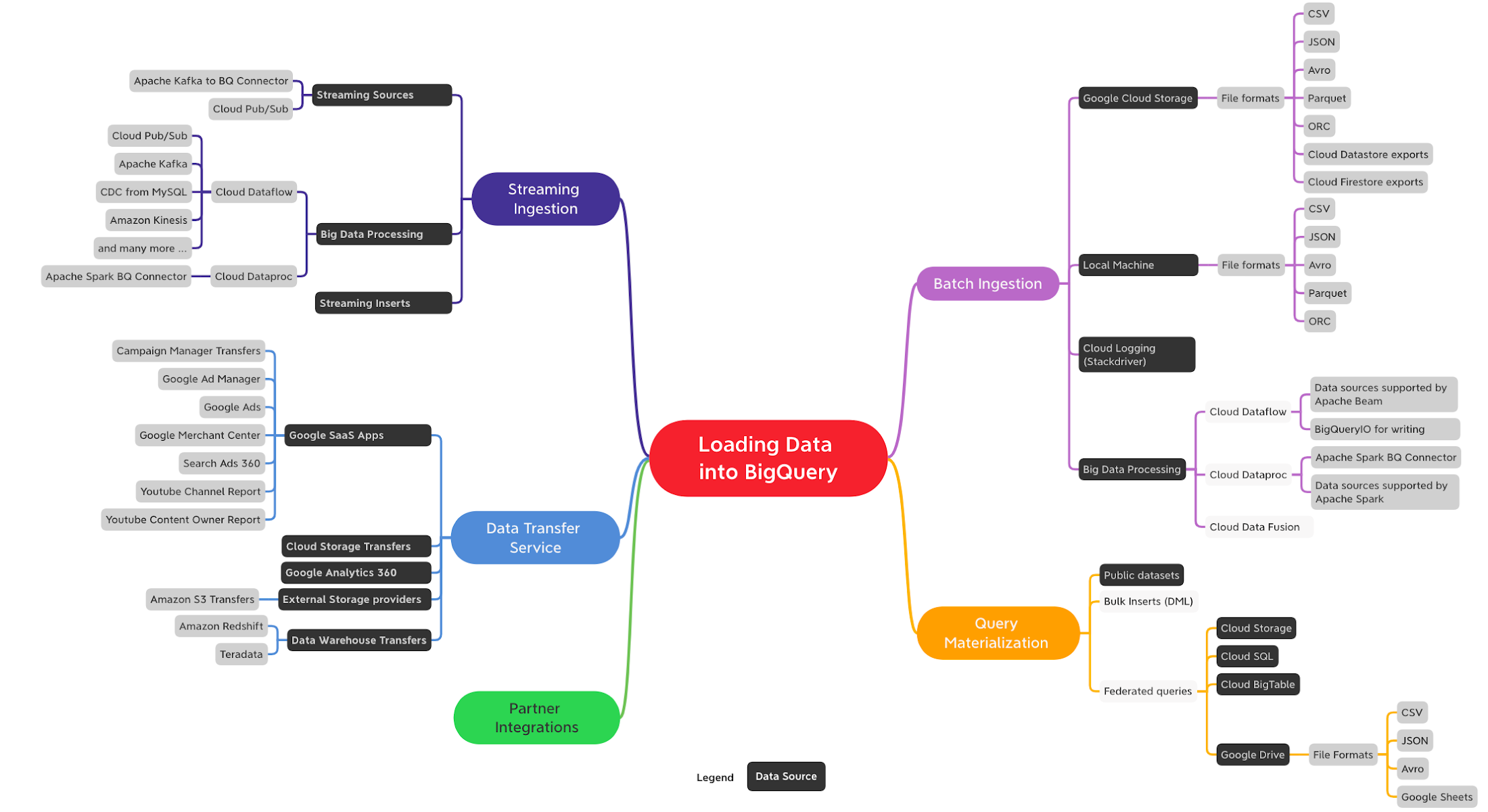
There are multiple ways to load data into BigQuery depending on data sources, data formats, load methods and use cases such as batch, streaming or data transfer. At a high level following are the ways you can ingest data into BigQuery:

• Batch Ingestion: Batch ingestion involves loading large, bounded, data sets that don’t have to be processed in real-time
• Streaming Ingestion: Streaming ingestion supports use cases that require analyzing high volumes of continuously arriving data with near-real-time dashboards and queries.
• Data Transfer Service (DTS): The BigQuery Data Transfer Service (DTS) is a fully managed service to ingest data from Google SaaS apps such as Google Ads, external cloud storage providers such as Amazon S3 and transferring data from data warehouse technologies such as Teradata and Amazon Redshift .
• Query Materialization: When you run queries in BigQuery their result sets can be materialized to create new tables.

source

Query without Loading (External Tables)

Using a federated query is one of the options to query external data sources directly without loading into BigQuery storage. You can query across Google services such as Google Sheets, Google Drive, Google Cloud Storage, Cloud SQL or Cloud BigTable without having to import the data into BigQuery.

You don’t need to load data into BigQuery before running queries in the following situations:

• Public Datasets: Public datasets are datasets stored in BigQuery and shared with the public.
• Shared Datasets: You can share datasets stored in BigQuery. If someone has shared a dataset with you, you can run queries on that dataset without loading the data.
• External data sources (Federated): You can skip the data loading process by creating a table based on an external data source.

Apart from the solutions available natively in BigQuery, you can also check data integration options from Google Cloud partners who have integrated their industry-leading tools with BigQuery.

To read more, please check here.

Check the following video for BQ best practices:

Here are some example queries in BQ which shows how to do partitioning and clustering on a public available dataset in BQ [ref]:

-- Query public available table
SELECT station_id, name FROM
    bigquery-public-data.new_york_citibike.citibike_stations
LIMIT 100;


-- Creating external table referring to gcs path
CREATE OR REPLACE EXTERNAL TABLE `taxi-rides-ny.nytaxi.external_yellow_tripdata`
OPTIONS (
  format = 'CSV',
  uris = ['gs://nyc-tl-data/trip data/yellow_tripdata_2019-*.csv', 'gs://nyc-tl-data/trip data/yellow_tripdata_2020-*.csv']
);

-- Check yello trip data
SELECT * FROM taxi-rides-ny.nytaxi.external_yellow_tripdata limit 10;

-- Create a non partitioned table from external table
CREATE OR REPLACE TABLE taxi-rides-ny.nytaxi.yellow_tripdata_non_partitoned AS
SELECT * FROM taxi-rides-ny.nytaxi.external_yellow_tripdata;


-- Create a partitioned table from external table
CREATE OR REPLACE TABLE taxi-rides-ny.nytaxi.yellow_tripdata_partitoned
PARTITION BY
  DATE(tpep_pickup_datetime) AS
SELECT * FROM taxi-rides-ny.nytaxi.external_yellow_tripdata;

-- Impact of partition
-- Scanning 1.6GB of data
SELECT DISTINCT(VendorID)
FROM taxi-rides-ny.nytaxi.yellow_tripdata_non_partitoned
WHERE DATE(tpep_pickup_datetime) BETWEEN '2019-06-01' AND '2019-06-30';

-- Scanning ~106 MB of DATA
SELECT DISTINCT(VendorID)
FROM taxi-rides-ny.nytaxi.yellow_tripdata_partitoned
WHERE DATE(tpep_pickup_datetime) BETWEEN '2019-06-01' AND '2019-06-30';

-- Let's look into the partitons
SELECT table_name, partition_id, total_rows
FROM `nytaxi.INFORMATION_SCHEMA.PARTITIONS`
WHERE table_name = 'yellow_tripdata_partitoned'
ORDER BY total_rows DESC;

-- Creating a partition and cluster table
CREATE OR REPLACE TABLE taxi-rides-ny.nytaxi.yellow_tripdata_partitoned_clustered
PARTITION BY DATE(tpep_pickup_datetime)
CLUSTER BY VendorID AS
SELECT * FROM taxi-rides-ny.nytaxi.external_yellow_tripdata;

-- Query scans 1.1 GB
SELECT count(*) as trips
FROM taxi-rides-ny.nytaxi.yellow_tripdata_partitoned
WHERE DATE(tpep_pickup_datetime) BETWEEN '2019-06-01' AND '2020-12-31'
  AND VendorID=1;

-- Query scans 864.5 MB
SELECT count(*) as trips
FROM taxi-rides-ny.nytaxi.yellow_tripdata_partitoned_clustered
WHERE DATE(tpep_pickup_datetime) BETWEEN '2019-06-01' AND '2020-12-31'
  AND VendorID=1;

Furthermore, if you are curious to know about internals of BQ, you can check here, here and also the following video.

Machine Learning in BigQuery

It is also possible to do machine learning in BigQuery instead of doing it outside of it. BigQuery ML increases development speed by eliminating the need to move data.

BigQuery ML supports the following types of models: [ref]

• Linear regression for forecasting; for example, the sales of an item on a given day. Labels are real-valued (they cannot be +/- infinity or NaN).
• Binary logistic regression for classification; for example, determining whether a customer will make a purchase. Labels must only have two possible values.
• Multiclass logistic regression for classification. These models can be used to predict multiple possible values such as whether an input is "low-value," "medium-value," or "high-value." Labels can have up to 50 unique values. In BigQuery ML, multiclass logistic regression training uses a multinomial classifier with a cross-entropy loss function.
• K-means clustering for data segmentation; for example, identifying customer segments. K-means is an unsupervised learning technique, so model training does not require labels nor split data for training or evaluation.
• Matrix Factorization for creating product recommendation systems. You can create product recommendations using historical customer behavior, transactions, and product ratings and then use those recommendations for personalized customer experiences.
• Time series for performing time-series forecasts. You can use this feature to create millions of time series models and use them for forecasting. The model automatically handles anomalies, seasonality, and holidays.
• Boosted Tree for creating XGBoost based classification and regression models.
• Deep Neural Network (DNN) for creating TensorFlow-based Deep Neural Networks for classification and regression models.
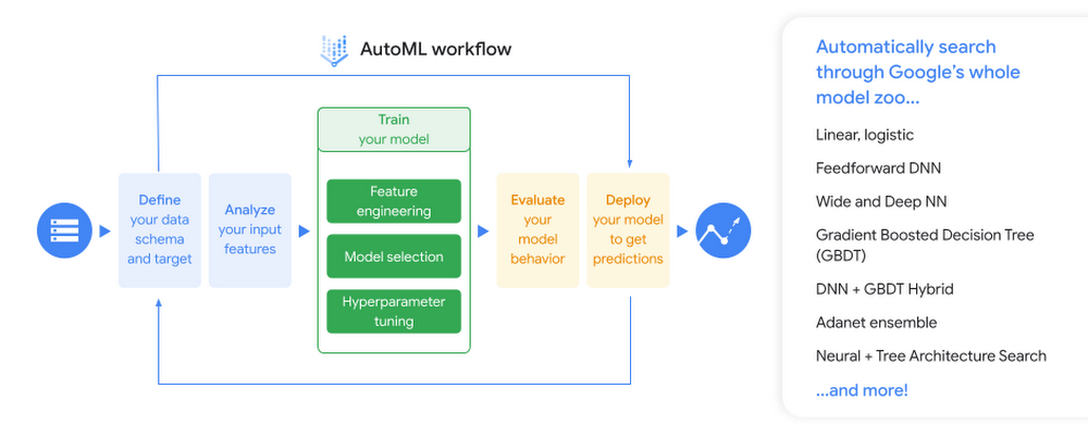
• AutoML Tables to create best-in-class models without feature engineering or model selection. AutoML Tables searches through a variety of model architectures to decide the best model.
• TensorFlow model importing. This feature lets you create BigQuery ML models from previously trained TensorFlow models, then perform prediction in BigQuery ML.
• Autoencoder for creating Tensorflow-based BigQuery ML models with the support of sparse data representations. The models can be used in BigQuery ML for tasks such as unsupervised anomaly detection and non-linear dimensionality reduction.

source

Check here and the following video to learn more about how to train a linear regression model in BQ:

Here is an example of training a liner regression model in BQ on the dataset we uploaded to GCS and BQ in the previous week using Airflow, and also how to do hyperparameter tuning: [ref1]

-- SELECT THE COLUMNS INTERESTED FOR YOU
SELECT passenger_count, trip_distance, PULocationID, DOLocationID, payment_type, fare_amount, tolls_amount, tip_amount
FROM `taxi-rides-ny.nytaxi.yellow_tripdata_partitoned` WHERE fare_amount != 0;

-- CREATE A ML TABLE WITH APPROPRIATE TYPE
CREATE OR REPLACE TABLE `taxi-rides-ny.nytaxi.yellow_tripdata_ml` (
`passenger_count` INTEGER,
`trip_distance` FLOAT64,
`PULocationID` STRING,
`DOLocationID` STRING,
`payment_type` STRING,
`fare_amount` FLOAT64,
`tolls_amount` FLOAT64,
`tip_amount` FLOAT64
) AS (
SELECT passenger_count, trip_distance, cast(PULocationID AS STRING), CAST(DOLocationID AS STRING),
CAST(payment_type AS STRING), fare_amount, tolls_amount, tip_amount
FROM `taxi-rides-ny.nytaxi.yellow_tripdata_partitoned` WHERE fare_amount != 0
);

-- CREATE MODEL WITH DEFAULT SETTING
CREATE OR REPLACE MODEL `taxi-rides-ny.nytaxi.tip_model`
OPTIONS
(model_type='linear_reg',
input_label_cols=['tip_amount'],
DATA_SPLIT_METHOD='AUTO_SPLIT') AS
SELECT
*
FROM
`taxi-rides-ny.nytaxi.yellow_tripdata_ml`
WHERE
tip_amount IS NOT NULL;

-- CHECK FEATURES
SELECT * FROM ML.FEATURE_INFO(MODEL `taxi-rides-ny.nytaxi.tip_model`);

-- EVALUATE THE MODEL
SELECT
*
FROM
ML.EVALUATE(MODEL `taxi-rides-ny.nytaxi.tip_model`,
(
SELECT
*
FROM
`taxi-rides-ny.nytaxi.yellow_tripdata_ml`
WHERE
tip_amount IS NOT NULL
));

-- PREDICT THE MODEL
SELECT
*
FROM
ML.PREDICT(MODEL `taxi-rides-ny.nytaxi.tip_model`,
(
SELECT
*
FROM
`taxi-rides-ny.nytaxi.yellow_tripdata_ml`
WHERE
tip_amount IS NOT NULL
));

-- PREDICT AND EXPLAIN
SELECT
*
FROM
ML.EXPLAIN_PREDICT(MODEL `taxi-rides-ny.nytaxi.tip_model`,
(
SELECT
*
FROM
`taxi-rides-ny.nytaxi.yellow_tripdata_ml`
WHERE
tip_amount IS NOT NULL
), STRUCT(3 as top_k_features));

-- HYPER PARAM TUNNING
CREATE OR REPLACE MODEL `taxi-rides-ny.nytaxi.tip_hyperparam_model`
OPTIONS
(model_type='linear_reg',
input_label_cols=['tip_amount'],
DATA_SPLIT_METHOD='AUTO_SPLIT',
num_trials=5,
max_parallel_trials=2,
l1_reg=hparam_range(0, 20),
l2_reg=hparam_candidates([0, 0.1, 1, 10])) AS
SELECT
*
FROM
`taxi-rides-ny.nytaxi.yellow_tripdata_ml`
WHERE
tip_amount IS NOT NULL;

After training the model, we need to deploy it. The following video explains how to that:

And here is the deployment steps: [ref1, ref2]

- gcloud auth login
- bq --project_id taxi-rides-ny extract -m nytaxi.tip_model gs://taxi_ml_model/tip_model
- mkdir /tmp/model
- gsutil cp -r gs://taxi_ml_model/tip_model /tmp/model
- mkdir -p serving_dir/tip_model/1
- cp -r /tmp/model/tip_model/* serving_dir/tip_model/1
- docker pull tensorflow/serving
- docker run -p 8501:8501 --mount type=bind,source=`pwd`/serving_dir/tip_model,target=
  /models/tip_model -e MODEL_NAME=tip_model -t tensorflow/serving &
- curl -d '{"instances": [{"passenger_count":1, "trip_distance":12.2, "PULocationID":"193", "DOLocationID":"264", "payment_type":"2","fare_amount":20.4,"tolls_amount":0.0}]}' -X POST http://localhost:8501/v1/models/tip_model:predict
- http://localhost:8501/v1/models/tip_model

Here is another nice blog post on using ML in BQ.

You can also check the following video which is a workshop on BQ+Airflow:

Other useful resources:

Amazon Redshift

Amazon Redshift is an alternate AWS data warehouse service that is not covered in the course but is quite comparable to BigQuery. It is an AWS Cloud-based petabyte-scale data warehouse solution that is completely managed. An Amazon Redshift data warehouse is a group of computer resources known as nodes that are arranged into a group known as a cluster. Each cluster contains one or more databases and is powered by an Amazon Redshift engine.

The following diagram illustrates a typical data processing flow in Amazon Redshift. [ref]

source

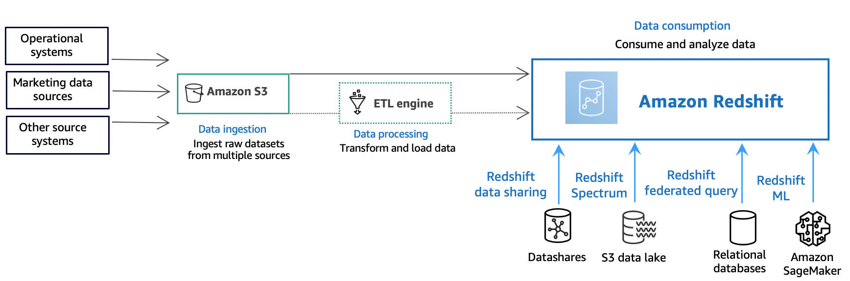
Different types of data sources constantly upload structured, semistructured, or unstructured data to the data storage layer at the data ingestion layer. This data storage area functions as a staging place for data in various states of consumption readiness. An Amazon Simple Storage Service (Amazon S3) bucket is an example of storage.

The source data is preprocessed, validated, and transformed utilizing extract, transform, load (ETL) or extract, load, transform (ELT) pipelines at the optional data processing layer. ETL techniques are subsequently used to refine these raw datasets. AWS Glue is an example of an ETL engine.

Data is imported into your Amazon Redshift cluster at the data consumption layer, where you can perform analytical applications.

Data can also be consumed for analytical workloads as follows:

• Use datashares to securely and easily transfer live data across Amazon Redshift clusters for reading purposes. Data can be shared at different levels, such as databases, schemas, tables, views, and SQL user-defined functions (UDFs).

• Amazon Redshift Spectrum may be used to query data in Amazon S3 files without having to load the data into Amazon Redshift tables. Amazon Redshift offers SQL capabilities designed for quick and online analytical processing (OLAP) of very big datasets stored in Amazon Redshift clusters and Amazon S3 data lakes.

• Using a federated query, you can join data from relational databases such as Amazon Relational Database Service (Amazon RDS), Amazon Aurora, or Amazon S3 with data from your Amazon Redshift database. Amazon Redshift can be used to query operational data directly (without moving it), apply transformations, and insert data into Amazon Redshift tables.

• Amazon Redshift machine learning (ML) generates models based on the data you provide and the metadata associated with the data inputs. Patterns in the incoming data are captured by these models. These models can be used to make predictions for new input data. Amazon Redshift works with Amazon SageMaker Autopilot to choose the best model and make the prediction function available in Amazon Redshift.

To learn more about Amazon Redshift and how to create database, tables, query data from Redshift or external sources check this and this tutorials. It's almost similar to BigQuery.

Let's check the more interesting part: Machine Learning in Redshift.

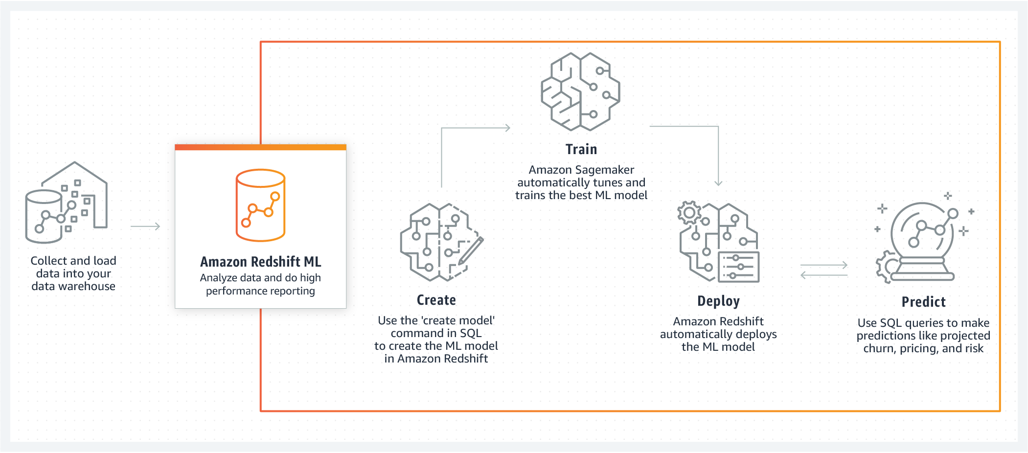
Machine Learning in Redshift

Amazon Redshift ML makes it simple for data analysts and database engineers to construct, train, and deploy machine learning models in Amazon Redshift data warehouses using standard SQL commands. You can use Redshift ML to access Amazon SageMaker, a fully managed machine learning service, without learning new tools or languages. Simply utilize SQL commands to develop and train Amazon SageMaker machine learning models on your Redshift data, and then use these models to predict.

source

Check the following demo to see how to do machine learning in Amazon Redshift:

Let's see how to create a model and running some inference queries for different scenarios using the SQL function that the CREATE MODEL command generates. [ref]

first create a table from a dataset in S3:

DROP TABLE IF EXISTS customer_activity;

CREATE TABLE customer_activity (
state varchar(2), 
account_length int, 
area_code int,
phone varchar(8), 
intl_plan varchar(3), 
vMail_plan varchar(3),
vMail_message int, 
day_mins float, 
day_calls int, 
day_charge float,
total_charge float,
eve_mins float, 
eve_calls int, 
eve_charge float, 
night_mins float,
night_calls int, 
night_charge float, 
intl_mins float, 
intl_calls int,
intl_charge float, 
cust_serv_calls int, 
churn varchar(6),
record_date date);

COPY customer_activity
FROM 's3://redshift-downloads/redshift-ml/customer_activity/'
REGION 'us-east-1' IAM_ROLE 'arn:aws:iam::XXXXXXXXXXXX:role/Redshift-ML'
DELIMITER ',' IGNOREHEADER 1;

Then creating the model.

CREATE MODEL customer_churn_auto_model FROM (
    SELECT 
        state,
        account_length,
        area_code,
        total_charge/account_length AS average_daily_spend, 
        cust_serv_calls/account_length AS average_daily_cases,
        churn 
    FROM 
        customer_activity
    WHERE  
        record_date < '2020-01-01' 
)
TARGET churn FUNCTION ml_fn_customer_churn_auto
IAM_ROLE 'arn:aws:iam::XXXXXXXXXXXX:role/Redshift-ML'SETTINGS (
  S3_BUCKET 'your-bucket'
);

The SELECT query creates the training data. The TARGET clause specifies which column is the machine learning label that the CREATE MODEL uses to learn how to predict. The remaining columns are the features (input) that are used for the prediction.

And finally, the prediction can be done as follows:

SELECT phone, 
       ml_fn_customer_churn_auto( 
          state,
          account_length,
          area_code, 
          total_charge/account_length , 
          cust_serv_calls/account_length )
          AS active FROM customer_activity WHERE record_date > '2020-01-01';

Conclusion

In this week, we focused more on data warehouses and reviewed Google BigQuery and Amazon Redshift services. We learned how to do normal SQL queries and also how to do machine learning in these warehouses using SQL.